Machine Learning with AdaBoost

What is Boosting?

From “The Boosting Approach to Machine Learning An Overview” by Roberrt E. Schapire,

Boosting, the machine-learning method that is the subject of this chapter, is based on the observation that finding many rough rules of thumb can be a lot easier than finding a single, highly accurate prediction rule. To apply the boosting approch, we start with a method or algorithm for finding the rough fules of thumb. The boosting algorithm calls this “weak” or “base” learning algorithm repeatedly, each time feeding it a different subset of the training examples(or, to be more precise, a different distribution or weighting over the training examples). Each time it is called, the base learning algorithm generates a new weak prediction rule, and after many rounds, the boosting algorithm must combine these weak rules into a single prediction rule that, hopefully, will be much more accurate than any one of the weak rules.

It is often discussed with bagging (bootstrap aggregation) because like bagging, boosting is a general approach that can be applied to many statistical learning methods for regression or classification.

There are many boosting algorithms.

That’s all very abstract. Let’s look at a specific example, walk step-by-step on how to apply boosting, and the definition above will start to make sense.

AdaBoost

Consider Adaboost, an acronym for adaptive boosting, developed in 1995 by Frund and Schapire. We will use AdaBoost on stumps, decision trees with only one split, but keep in mind that boosting can be used on any machine learning method. Stumps are just always used for illustrative purposes.

Let say we are given a training set

$x_{i}$ could represent an email message and $y_{i} = -1$ if it is not spam and $y_{i} = 1$ if it is spam. Note that we are working in a two-class setting for simplicity. We can generalize to multi-class scenarios.

Let’s assume we have T weak classifiers and a scalar constant $α_{t}$ associated with each

Let

Define the strong classifier as the sign of this inner product

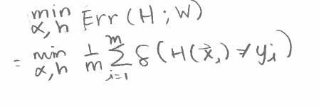
The objective is to choose $h$ and $α$ to minimize the empirical classification error of $H(\vec{x})$

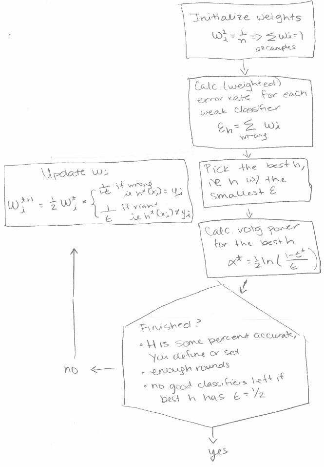
AdaBoost Algorithm

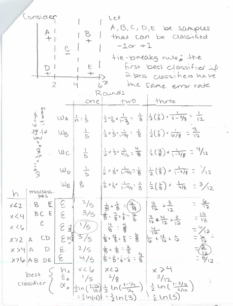
Example of AdaBoost

This is long but clear. I recommend speeding up the video so that then it probably will not take 55 minutes to watch the video.

Here is the walk-thru example on the board written down.

Reasoning Behind AdaBoost

Now, why does sometimes AdaBoost work. What were the developers thinking?

The Crowd Is Smarter Than Its Parts

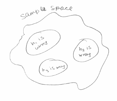
Let say this is our classifier $H(\vec{x}) = sign(h_{1}(x) + h_{2}(x) + h_{3}(x))$ .
The image below is of the sample space and where each weak classifier is wrong. In this case, $H(\vec{x})$ is 100% accurate in the sample space. The idea is that we can get a strong classifier using weak classifiers that are wrong in different cases and the smarter crowd can outweigh individual bad classifiers.

Exaggerate Errors in Previous Weak Classifiers When Constructing Next Classifier

We do not want the cases where our weak classifiers are wrong to overlap. Initially, when calculating our error rate, each sample carries the same weight $1/n$ . We will update these weights so that in our next iteration, when we calculate the error rate, the samples where the previous classifier misclassified are weighted more.

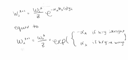
$z$ is the normalizing factor. It is there so that $Σw_{i} = 1$ ie $W$ is a distribution. We call this enforcing a distribution. A distribution is a set of weights that sum up to 1. This is not exactly the formula written above but they are equivalent. The formulas above are easier to work with. The reasons for walking through how this formula is equivalent to the easier formulas are pedagogical.

Properties Of This Formula That We Need

Notice that using this formula

samples that were wrong in our previously chosen weak classifiers to be included in our strong classifer are weighed more.
the weights follow a distribution

But Why This Formula?

There are an infinite number for formulas that would satisfy the aforementioned requirements. Prof. Patrick Winston asked Schapire, who came up with this formula, how he came up with this formula. “And the answer is it did not spring from the heart of a mathematician in the first ten minutes that he looked at this problem… he[Schapire] was thinking about this on his couch for about a year and his wife was getting pretty sore. But he finally found it and saved their marriage. So where does stuff like this come from? Really, it comes from knowing a lot of mathematics, and seeing a lot of situations and knowing that something like this might be mathematically convenient.”
And it is mathematically convenient. Read my post on why Euler’s number e is so special. There are nice properties that Schapire did not realize such as the fact that this formula leads to

$\sum\limits_{wrong}w_{i, t} = \sum\limits_{right}w_{i, t} = 1/2$

That was not on purpose!

Solving The Problem of Weak Classifiers’ Errors Still Overlapping

It doesn’t always have to be so simple. It can be like this.

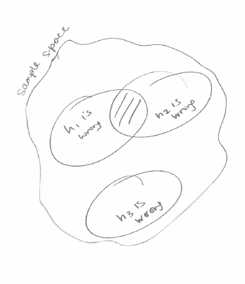
We solve this problem by weighing h3 more than the weights of h1 and h2 combined. In our equation, that means

We use coefficents/weights/alphas that minimize the error rate of our strong classifier. This is a Calculus problem.

We want to minimize Err(H) = $l(H)$ .

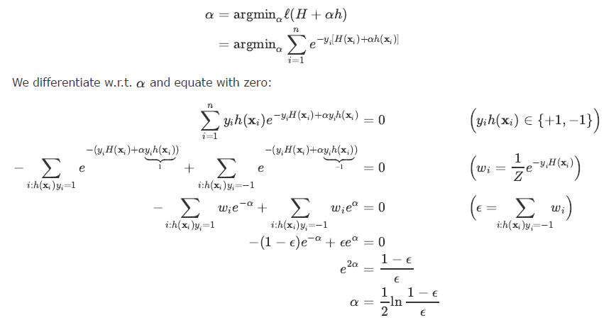
Error Rate Has An Upper Bound

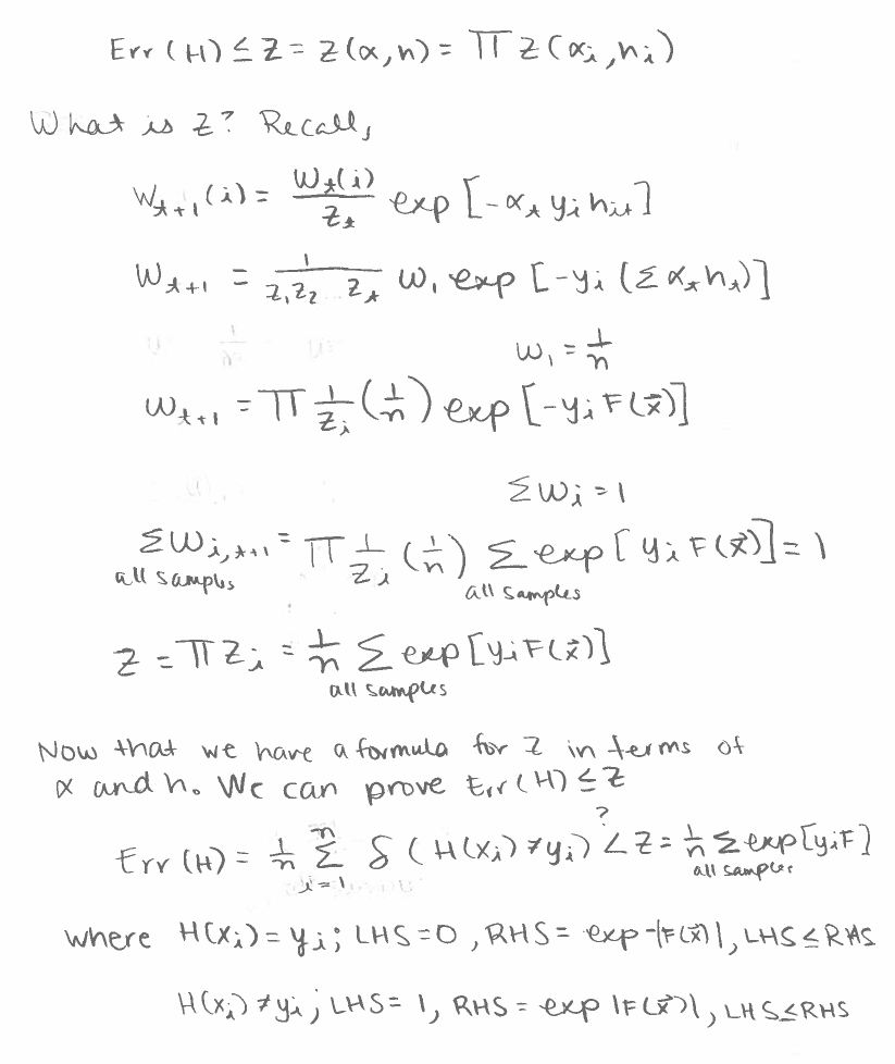
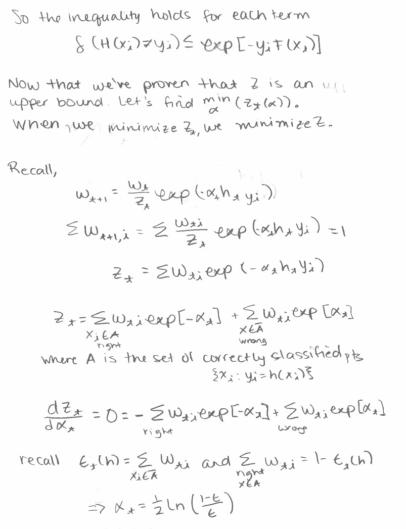
Another fact about about adaboost is that its error rate has an upper bound. The following is a derivation of the upper bound. First, we need to prove that $Z$ is an upper bound, ie

AdaBoost using Sci-Kit Learn

learning_rate is simple r in α = rln((1-e/e)). This just means that $w_{t+1} = w_{t}/z * exp(-2/r * αhy)$ Everything above still holds.

from sklearn.ensemble import AdaBoostClassifier
from sklearn.tree import DecisionTreeClassifier

import numpy as np
X = np.array([[1], [1], [3], [5], [5]]); y = np.array([1, 1, -1, 1, 1])

stump = DecisionTreeClassifier(max_depth = 1)
bdt = AdaBoostClassifier(stump, n_estimators = 999, learning_rate = 0.5)

bdt.fit(X, y)

AdaBoostClassifier(algorithm='SAMME.R',
          base_estimator=DecisionTreeClassifier(class_weight=None, criterion='gini', max_depth=1,
            max_features=None, max_leaf_nodes=None,
            min_impurity_decrease=0.0, min_impurity_split=None,
            min_samples_leaf=1, min_samples_split=2,
            min_weight_fraction_leaf=0.0, presort=False, random_state=None,
            splitter='best'),
          learning_rate=0.5, n_estimators=999, random_state=None)

bdt.predict(X)

array([ 1,  1, -1,  1,  1])

array([ 1,  1, -1,  1,  1])

array([[1],
       [1],
       [3],
       [5],
       [5]])