Decision Trees and Random Forests on Titanic Data
import pandas as pd
import seaborn as sns
import matplotlib.pyplot as plt
from sklearn.impute import SimpleImputer
from sklearn import tree
from sklearn.preprocessing import OneHotEncoder
import graphviz
from sklearn.ensemble import RandomForestClassifier
Load Data
raw_train = train = pd.read_csv('../../src/train.csv', index_col= 'PassengerId')
train = raw_train.copy()
train.head()
| Survived | Pclass | Name | Sex | Age | SibSp | Parch | Ticket | Fare | Cabin | Embarked | |
|---|---|---|---|---|---|---|---|---|---|---|---|
| PassengerId | |||||||||||
| 1 | 0 | 3 | Braund, Mr. Owen Harris | male | 22.0 | 1 | 0 | A/5 21171 | 7.2500 | NaN | S |
| 2 | 1 | 1 | Cumings, Mrs. John Bradley (Florence Briggs Th... | female | 38.0 | 1 | 0 | PC 17599 | 71.2833 | C85 | C |
| 3 | 1 | 3 | Heikkinen, Miss. Laina | female | 26.0 | 0 | 0 | STON/O2. 3101282 | 7.9250 | NaN | S |
| 4 | 1 | 1 | Futrelle, Mrs. Jacques Heath (Lily May Peel) | female | 35.0 | 1 | 0 | 113803 | 53.1000 | C123 | S |
| 5 | 0 | 3 | Allen, Mr. William Henry | male | 35.0 | 0 | 0 | 373450 | 8.0500 | NaN | S |
Counting Number of Unique Values for Each Feature
Name is Unique So We Are Dropping It
A column with unique values has no predictive value. It can be used as an index, but we are not using it as an index. We already have an index.
Recall that our training set has 891 rows.
for f in train:
    n_dups = len(train[f].unique())
    print(f, n_dups)
Survived 2
Pclass 3
Name 891
Sex 2
Age 89
SibSp 7
Parch 7
Ticket 681
Fare 248
Cabin 148
Embarked 4
train = train.drop(columns=['Name'])
Ticket and Cabin are Categorical Features with Many Unique Values
Recall that a categorical feature with only unique values has no predictive value. It makes sense then that a feature with a large number of unique values relative to the number of rows has little predictive value if any. Ticket and Cabin may have little to no predictive value for this reason. Let’s look at Ticket and Cabin closer.
Ticket Doesn’t Appear Useful
pd.options.display.max_rows = 12
train.Ticket.value_counts()
347082      7
1601        7
CA. 2343    7
CA 2144     6
3101295     6
347088      6
           ..
29105       1
PC 17473    1
113056      1
323951      1
27267       1
345364      1
Name: Ticket, Length: 681, dtype: int64
train = train.drop(columns=['Ticket'])
Cabin Probably Not Useful
Let’s drop Cabin. The letters at the front of cabin values may be useful, but probably not. 25% of the data are nulls. The letters are probably correlated with wealth, socio-economic status and we already know that with PClass. If our models are not effective, we can just try using Cabin later.
train.Cabin.value_counts()
B96 B98        4
C23 C25 C27    4
G6             4
F33            3
C22 C26        3
E101           3
              ..
E31            1
A14            1
B3             1
A6             1
C30            1
B86            1
Name: Cabin, Length: 147, dtype: int64
cabin_grp = train.Cabin.str[0]
cabin_grp.value_counts()
C    59
B    47
D    33
E    32
A    15
F    13
G     4
T     1
Name: Cabin, dtype: int64
n_nan_cg = cabin_grp.count(); n_nan_cg
204
train = train.drop(columns = ['Cabin'])
Identifying Numerical and Categorical Variables
target = 'Survived'

is_num = train.dtypes\
        .apply(lambda x: x == 'float64' or x == 'int64')
num_cols = train.dtypes.index[is_num]
num_f = set(num_cols) - {target}
num_f
{'Age', 'Fare', 'Parch', 'Pclass', 'SibSp'}
cat_f = set(train.columns) - num_f - {target}
cat_f
{'Embarked', 'Sex'}
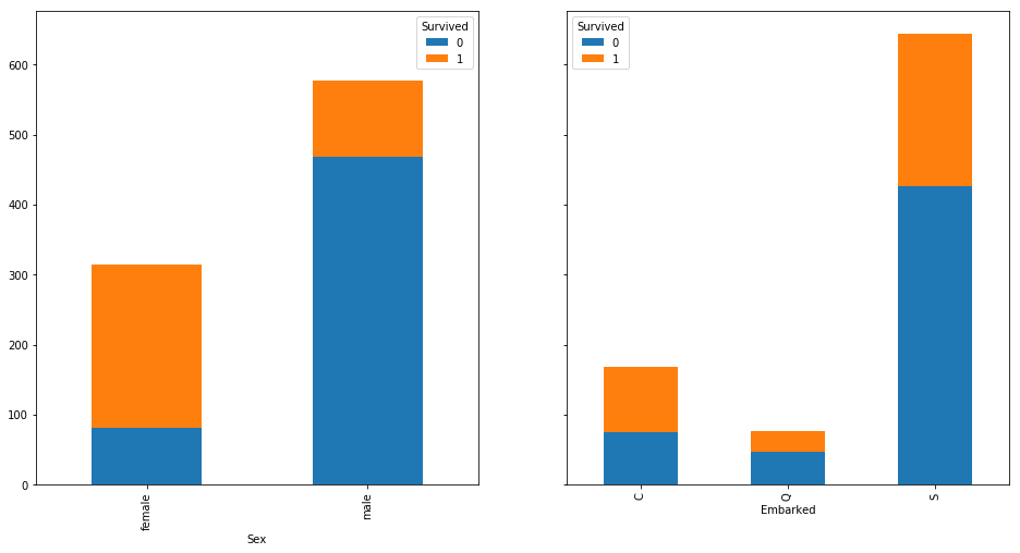
fig, axes = plt.subplots(nrows = 1, ncols = len(cat_f),
                         figsize = (16,8),
                         sharey = True)

for i, f in enumerate(cat_f):
    pd.crosstab(train[f], train['Survived'])\
        .plot(kind = 'bar', stacked = True, ax = axes[i])

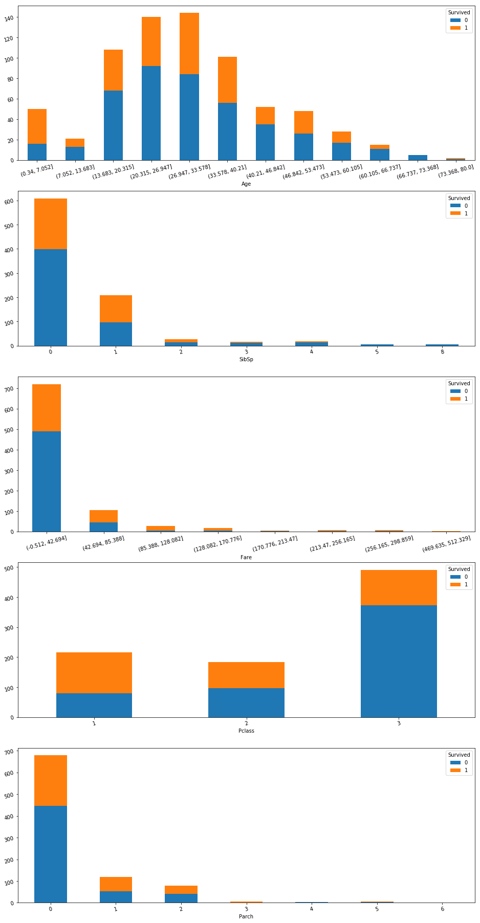
fig, axes = plt.subplots(nrows = len(num_f), ncols = 1,
                         figsize = (16,28))

for i, f in enumerate(num_f):
    f_col = train[f].copy()
    if len(train[f].unique()) > 7:
        f_col = pd.cut(train[f], 12)

    ax = axes[i]
    subplot = pd.crosstab(f_col, train['Survived'])\
            .plot(kind = 'bar', stacked = True, ax = ax,
                 fontsize = 15)
    ax.tick_params(labelrotation = 15, labelsize = 10)
    plt.rc('axes', labelsize = 10)
    plt.subplots_adjust(bottom = 0.01)

Note About Not Deskewing Data
Note that although Parch, Fare, and SibSp are highly skewed, we do not need to deskew those features because skewed distributions are not harmful to decision tree models. In fact it can be harmful because deskewing the model can prevent splitting at very high or low points.
Imputing Nans
Let’s keep this simple. We will impute nans for categorical variables with the mode and for numarical variables the mean.
X = train.drop(columns=['Survived']).copy(); y = train.Survived.copy()
X.isnull().sum().sum()
179
num_f = list(num_f); cat_f = list(cat_f)
imp_X = X.copy()
cat_imp = SimpleImputer(strategy='most_frequent')
num_imp = SimpleImputer(strategy='mean')
imp_X[cat_f] = cat_imp.fit_transform(imp_X[cat_f])
imp_X[num_f] = num_imp.fit_transform(imp_X[num_f])
imp_X.isnull().sum().sum()
0
dumm_X = pd.get_dummies(imp_X); dumm_X.head(3)
| Pclass | Age | SibSp | Parch | Fare | Sex_female | Sex_male | Embarked_C | Embarked_Q | Embarked_S | |
|---|---|---|---|---|---|---|---|---|---|---|
| PassengerId | ||||||||||
| 1 | 3.0 | 22.0 | 1.0 | 0.0 | 7.2500 | 0 | 1 | 0 | 0 | 1 |
| 2 | 1.0 | 38.0 | 1.0 | 0.0 | 71.2833 | 1 | 0 | 1 | 0 | 0 |
| 3 | 3.0 | 26.0 | 0.0 | 0.0 | 7.9250 | 1 | 0 | 0 | 0 | 1 |
Preparing Test Set
test = pd.read_csv('../../src/test.csv', index_col='PassengerId')
test.head()
| Pclass | Name | Sex | Age | SibSp | Parch | Ticket | Fare | Cabin | Embarked | |
|---|---|---|---|---|---|---|---|---|---|---|
| PassengerId | ||||||||||
| 892 | 3 | Kelly, Mr. James | male | 34.5 | 0 | 0 | 330911 | 7.8292 | NaN | Q |
| 893 | 3 | Wilkes, Mrs. James (Ellen Needs) | female | 47.0 | 1 | 0 | 363272 | 7.0000 | NaN | S |
| 894 | 2 | Myles, Mr. Thomas Francis | male | 62.0 | 0 | 0 | 240276 | 9.6875 | NaN | Q |
| 895 | 3 | Wirz, Mr. Albert | male | 27.0 | 0 | 0 | 315154 | 8.6625 | NaN | S |
| 896 | 3 | Hirvonen, Mrs. Alexander (Helga E Lindqvist) | female | 22.0 | 1 | 1 | 3101298 | 12.2875 | NaN | S |
test = test[X.columns]
test.head(2)
| Pclass | Sex | Age | SibSp | Parch | Fare | Embarked | |
|---|---|---|---|---|---|---|---|
| PassengerId | |||||||
| 892 | 3 | male | 34.5 | 0 | 0 | 7.8292 | Q |
| 893 | 3 | female | 47.0 | 1 | 0 | 7.0000 | S |
test.isnull().sum().sum()
87
test[cat_f] = cat_imp.transform(test[cat_f])
test[num_f] = num_imp.transform(test[num_f])
test.isnull().sum().sum()
0
def get_test_dummies(test_df, X_dummies):
    test_dummies = pd.get_dummies(data = test_df)

    # There may be values for categorical features in the training set and not in the test set.
    values_not_in_test_dummies = set(X_dummies.columns) - set(test_dummies.columns)
    for v in values_not_in_test_dummies:
        test_dummies[v] = 0
    test_dummies.shape
    # Values not in the training set, but are in the test set.
    # Eg The range of GarageCars in the training set is [1,4];
    # The test set may have a house with more than four cars
    values_not_in_X = set(test_dummies.columns) - set(X_dummies.columns)
    test_dummies = test_dummies.drop(columns = list(values_not_in_X))

    col_order = X_dummies.columns.tolist()
    test_dummies = test_dummies[col_order]

    return test_dummies

dumm_test = get_test_dummies(test, dumm_X)
dumm_test.isnull().sum()
Pclass        0
Age           0
SibSp         0
Parch         0
Fare          0
Sex_female    0
Sex_male      0
Embarked_C    0
Embarked_Q    0
Embarked_S    0
dtype: int64
Decision Tree Classifier
Decison trees are not very accurate. They are prone to overfitting.
Random forests, however, can be powerful.
dtree = tree.DecisionTreeClassifier()
dtree.fit(dumm_X, y)

ff = dumm_X.columns
dot_data = tree.export_graphviz(dtree, out_file=None,
                               feature_names = ff)
graph = graphviz.Source(dot_data)

graph
predictions = pd.DataFrame({'Survived': dtree.predict(dumm_test)},
                           index = dumm_test.index)

predictions.to_csv('dtree-naive-predictions.csv')
Kaggle accuracy = 0.727272; 9837th place out of 10736
>>> clf = RandomForestClassifier(n_estimators=100, max_depth=2,
...                              random_state=0)
>>> clf.fit(X, y)
RandomForestClassifier(bootstrap=True, class_weight=None, criterion='gini',
            max_depth=2, max_features='auto', max_leaf_nodes=None,
            min_impurity_decrease=0.0, min_impurity_split=None,
            min_samples_leaf=1, min_samples_split=2,
            min_weight_fraction_leaf=0.0, n_estimators=100, n_jobs=None,
            oob_score=False, random_state=0, verbose=0, warm_start=False)
>>> print(clf.feature_importances_)
[0.14205973 0.76664038 0.0282433  0.06305659]
>>> print(clf.predict([[0, 0, 0, 0]]))
[1]
rf = RandomForestClassifier(n_estimators = 50 )
rf.fit(dumm_X, y)

predictions = pd.DataFrame({'Survived': rf.predict(dumm_test)},
                           index = dumm_test.index)

predictions.to_csv('rf-predictions.csv')
RandomForestClassifier(bootstrap=True, class_weight=None, criterion='gini',
            max_depth=None, max_features='auto', max_leaf_nodes=None,
            min_impurity_decrease=0.0, min_impurity_split=None,
            min_samples_leaf=1, min_samples_split=2,
            min_weight_fraction_leaf=0.0, n_estimators=50, n_jobs=None,
            oob_score=False, random_state=None, verbose=0,
            warm_start=False)
Kaggle score 0.74162 which is unsurprisingly an improvement
rf100 = RandomForestClassifier(n_estimators = 100 )
rf100.fit(dumm_X, y)

predictions = pd.DataFrame({'Survived': rf100.predict(dumm_test)},
                           index = dumm_test.index)

predictions.to_csv('rf100-predictions.csv')
score improved to 0.76076
Is An Accuracy of 0.76076 Good?
Not really. It’s more accurate than guessing that every passenger died. 61% of passengers died so that method would be 61% accurate. However, if we just guessed that every female passenger survived and every male passenger died, we would be accurate 78.6% of the time, more than 76% of the time, the accurac of our best random forest.
pd.crosstab(train.Sex, train.Survived, normalize = 'all')
| Survived | 0 | 1 |
|---|---|---|
| Sex | ||
| female | 0.090909 | 0.261504 |
| male | 0.525253 | 0.122334 |
0.261+0.525
0.786
How Can We Do Better?
We can improve our XG Boost or Ada boost and compare which decision tree produces better results.