
Decision Trees And Random Forests
What are decision trees?
According to Introduction to Statistical Learning 7th edition
tree based methods for regression and classification… involve stratifying or segmenting the predictor space into a number of simple regions… since the set of splitting rules used to segment the predictor space can be summarized in a tree, these types of approaches are known as decision tree methods.
Decision trees are one of those things better explained and defined with a picture.
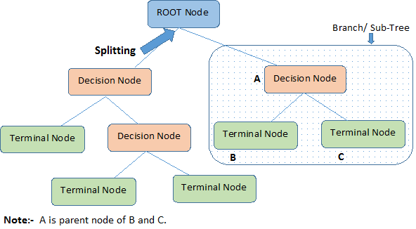
What are these decision tree methods?
Decision trees can be categorized by (1) the algorithm used to build it and (2) whether the tree is applied to a regression or classification problem.
Algorithms for Building Decision Trees
There are many decision tree algorithms. They include ID3 (Iterative Dichotomizer 3), C4.5, CART (Classification and Regression Tree), CHAID, QUEST, GUIDE, CRUISE, and CTREE. The three most common are ID3, C4.5, and CART.
This guide will focus on CART. Coincidentally, sklearn also uses CART.
Classification Trees
Let’s walk through how to to build a classification tree, that is a decision tree where the target variable is a categorical variable, using CART. Our example dataset will be a very, very small sample of the Titanic data set. The dataset is of people who boarded the Titanic. Our target variable is whether a passenger survived the Titanic.
The attributes are Pclass, Sex, Age, and Survived. We say the possible values are upper, middle, lower, female, etc.
import pandas as pd
from sklearn import tree
import warnings; warnings.filterwarnings('ignore')

train = pd.read_csv('../../src/train.csv')
train = train.set_index('PassengerId')

toy_feats = ['Pclass', 'Sex', 'Age']

seed = 2
toy = train[toy_feats + ['Survived']].sample(n = 5, random_state = seed)

ec_class = {1:'upper', 2:'middle', 3:'lower'}
for old, new in ec_class.items():
    toy.Pclass[toy.Pclass == old] = new

toy
| Pclass | Sex | Age | Survived | |
|---|---|---|---|---|
| PassengerId | ||||
| 708 | upper | male | 42.0 | 1 |
| 38 | lower | male | 21.0 | 0 |
| 616 | middle | female | 24.0 | 1 |
| 170 | lower | male | 28.0 | 0 |
| 69 | lower | female | 17.0 | 1 |
How do we split our root node?
Let’s take a small detour and consider this data set.
pd.DataFrame({'dates': ['1/2/18', '3/12/18', '8/3/18'],
              'weather': ['cold', 'cold', 'hot'],
              'doIeatIceCream': ['no', 'no', 'yes']})
| dates | weather | doIeatIceCream | |
|---|---|---|---|
| 0 | 1/2/18 | cold | no |
| 1 | 3/12/18 | cold | no |
| 2 | 8/3/18 | hot | yes |
The decision tree for this dataset is obvious. The answer is obvious because the nodes for hot and cold weather are pure, ie I ate icream on all hot days and did not on cold days.
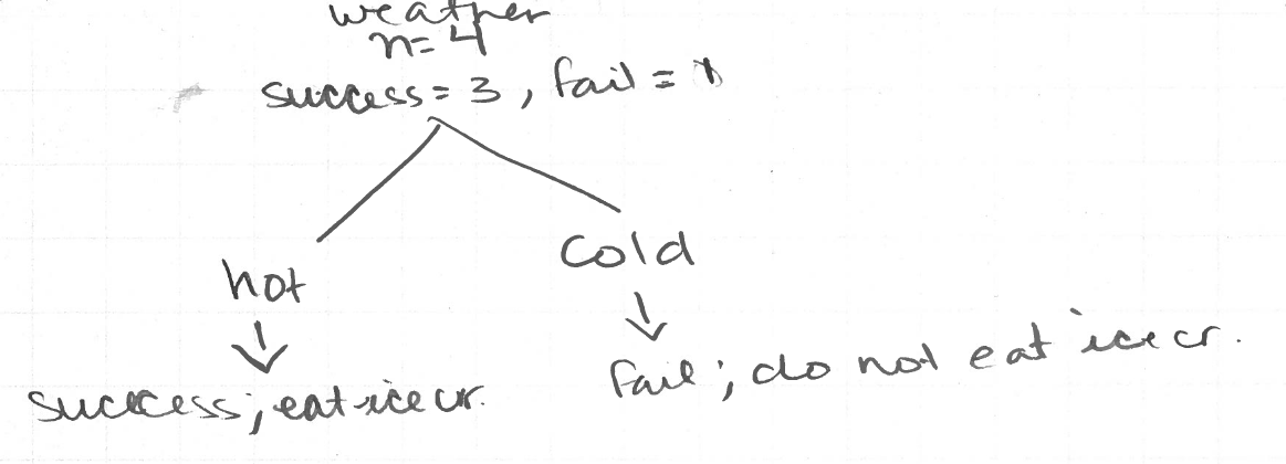
Now let’s return to the Titanic dataset. ID3, CART, and C4.5 split based on purity. The differences are how many nodes are in a split and how purity is measured. CART only creates binary trees meaning one split only has two nodes.
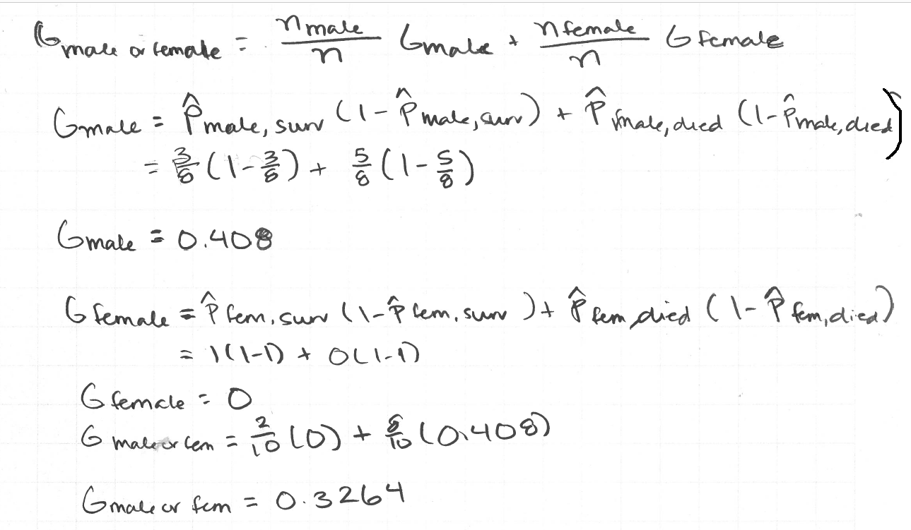
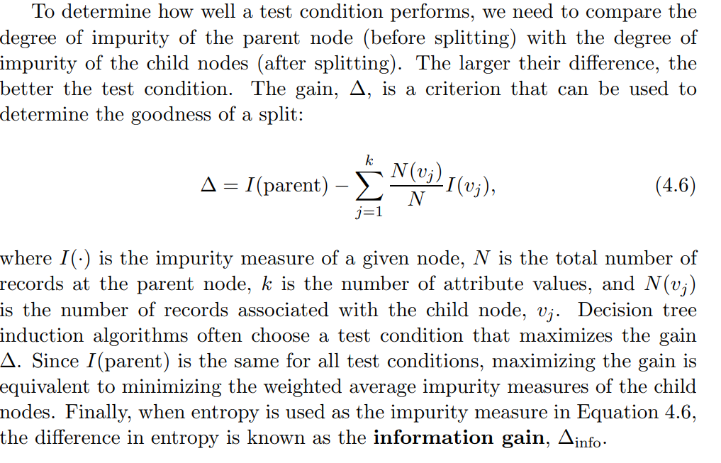
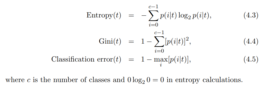
To measure purity, CART uses the gini index or towing index. We will use the gini index because it is easier. We need to find the gini index for every possible split and pick the split with the lowest gini index. A smaller gini index indicates more purity, less impurity.
Gini Index
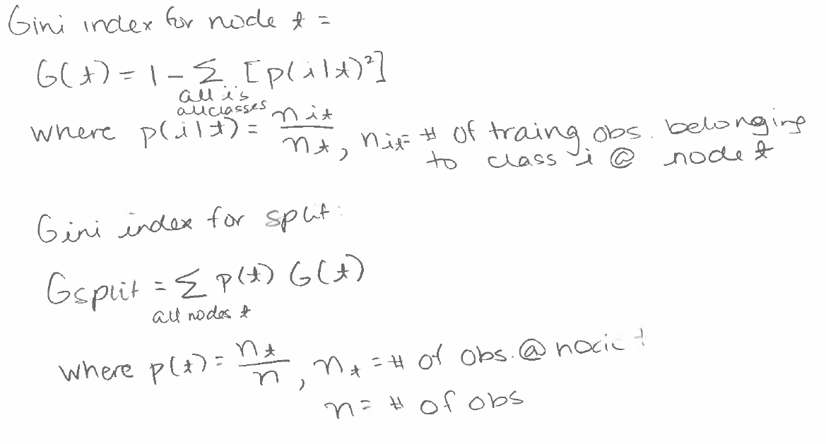
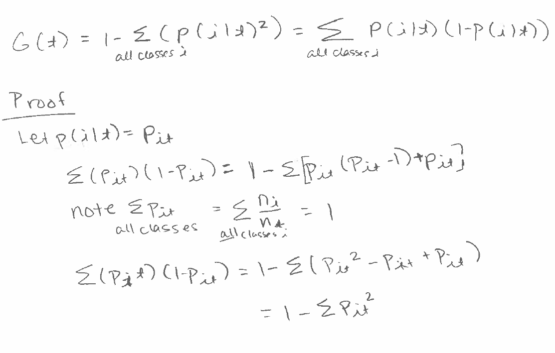
Sometimes, the Gini index is written another way. This is the proof that the two formulas are equal.
Binary Variables
Let’s calculate the Gini index for the male node, female node, and finally the split on Sex.
Categorical Variables
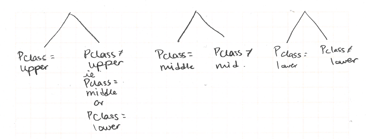
Recall that CART only does binary splits. We cannot do a three-way split for the Pclass variable. We can only do a split where one branch is for one or two values and the other branch is not those values.
We need to find Gini indices for the following possible splits:
Here is how to calculate the Gini index for split to is upper class and is not upper class.
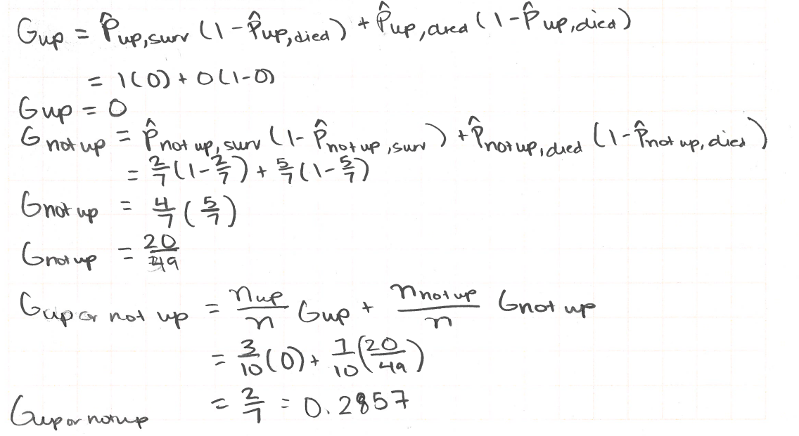
As you can see, this is a very tedious process. Fortunately, sklearn can build our tree for us. Unfortunately, sklearn does not support tree pruning.
from sklearn import tree
dumm = pd.get_dummies(toy)
clf = tree.DecisionTreeClassifier()
clf = clf.fit(dumm.drop(columns = ['Survived']), dumm.Survived)
clf
DecisionTreeClassifier(class_weight=None, criterion='gini', max_depth=None,
            max_features=None, max_leaf_nodes=None,
            min_impurity_decrease=0.0, min_impurity_split=None,
            min_samples_leaf=1, min_samples_split=2,
            min_weight_fraction_leaf=0.0, presort=False, random_state=None,
            splitter='best')
ff = list(set(dumm.columns) - {'Survived'})
dot_data = tree.export_graphviz(clf, out_file=None,
                                feature_names = ff
                               )
graph = graphviz.Source(dot_data)
Tree Pruning
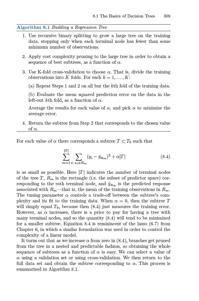
If we stopped here, we would get very good predictions on the training set, but probably not on the test set. Decision trees in particular suffer from overfitting. We should prune our decision tree. (To prune an actual tree or bush is to trim it.) CART uses cost complexity pruning also known as weakest link pruning. From Introduction to Statistical Learning 7th edition, when using cost complexity pruning, “rather than considering every possible subree [as we do in cross-validation], we consider a sequence of trees indexed by a nonnegative tuning parameter α.
Notes About Using sklearn to Build Decision Trees
sklearn is missing many functionalities. It only implements the CART algorithm. It “does not support categorical variables for now.” Note that we had to one-hot encode our dataframe before providing it as an argument in sklearn’s tree function. If Pclass had more than three values, then just one-hot encoding would not have been enough to build a decision tree with categorical variables. We would need to create columns for when a row takes on one of two values of an attribute.
Consider this dataset where Pclass has four values, not three.
new_toy = toy.append(pd.DataFrame({'Pclass': ['dirt_poor'], 'Sex': ['female'], 'Age':[40], 'Survived': [0]}))
new_toy
| Pclass | Sex | Age | Survived | |
|---|---|---|---|---|
| 708 | upper | male | 42.0 | 1 |
| 38 | lower | male | 21.0 | 0 |
| 616 | middle | female | 24.0 | 1 |
| 170 | lower | male | 28.0 | 0 |
| 69 | lower | female | 17.0 | 1 |
| 0 | dirt_poor | female | 40.0 | 0 |
dummies = pd.get_dummies(new_toy); dummies
| Age | Survived | Pclass_dirt_poor | Pclass_lower | Pclass_middle | Pclass_upper | Sex_female | Sex_male | |
|---|---|---|---|---|---|---|---|---|
| 708 | 42.0 | 1 | 0 | 0 | 0 | 1 | 0 | 1 |
| 38 | 21.0 | 0 | 0 | 1 | 0 | 0 | 0 | 1 |
| 616 | 24.0 | 1 | 0 | 0 | 1 | 0 | 1 | 0 |
| 170 | 28.0 | 0 | 0 | 1 | 0 | 0 | 0 | 1 |
| 69 | 17.0 | 1 | 0 | 1 | 0 | 0 | 1 | 0 |
| 0 | 40.0 | 0 | 1 | 0 | 0 | 0 | 1 | 0 |
Passing in a dummied dataframe with the Sex_female column would effectively give us the same decision tree as passing in a dataframe without Sex_female
dummies = dummies.drop(columns=['Sex_female']); dummies.head()
| Age | Survived | Pclass_dirt_poor | Pclass_lower | Pclass_middle | Pclass_upper | Sex_male | |
|---|---|---|---|---|---|---|---|
| 708 | 42.0 | 1 | 0 | 0 | 0 | 1 | 1 |
| 38 | 21.0 | 0 | 0 | 1 | 0 | 0 | 1 |
| 616 | 24.0 | 1 | 0 | 0 | 1 | 0 | 0 |
| 170 | 28.0 | 0 | 0 | 1 | 0 | 0 | 1 |
| 69 | 17.0 | 1 | 0 | 1 | 0 | 0 | 0 |
This is why we did not need to add a Pclass_lowVmid column and the like. We already have Pclass_upper and that’s enough. However, if Pclass had four variables, our dummied dataframe would not have enough columns to make a decision tree with categorical variables. We can easily make a work-around so that sklearn can handle categorical variables.
dummies['Pclass_dirtVlow'] = dummies.Pclass_dirt_poor + dummies.Pclass_lower
dummies['Pclass_dirtVmid'] = dummies.Pclass_dirt_poor + dummies.Pclass_middle
dummies['Pclass_dirtVup'] = dummies.Pclass_dirt_poor + dummies.Pclass_upper

dummies['Pclass_lowVmid'] = dummies.Pclass_lower + dummies.Pclass_middle
dummies['Pclass_lowVup'] = dummies.Pclass_lower + dummies.Pclass_upper

dummies['Pclass_midVup'] = dummies.Pclass_middle + dummies.Pclass_upper
dummies.head()
| Age | Survived | Pclass_dirt_poor | Pclass_lower | Pclass_middle | Pclass_upper | Sex_male | Pclass_dirtVlow | Pclass_dirtVmid | Pclass_dirtVup | Pclass_lowVmid | Pclass_lowVup | Pclass_midVup | |
|---|---|---|---|---|---|---|---|---|---|---|---|---|---|
| 708 | 42.0 | 1 | 0 | 0 | 0 | 1 | 1 | 0 | 0 | 1 | 0 | 1 | 1 |
| 38 | 21.0 | 0 | 0 | 1 | 0 | 0 | 1 | 1 | 0 | 0 | 1 | 1 | 0 |
| 616 | 24.0 | 1 | 0 | 0 | 1 | 0 | 0 | 0 | 1 | 0 | 1 | 0 | 1 |
| 170 | 28.0 | 0 | 0 | 1 | 0 | 0 | 1 | 1 | 0 | 0 | 1 | 1 | 0 |
| 69 | 17.0 | 1 | 0 | 1 | 0 | 0 | 0 | 1 | 0 | 0 | 1 | 1 | 0 |
Other Measures of Purity
Entropy

where $p̂_{mk}$ is the proportion of training observations in the mth region that are from the kth class.
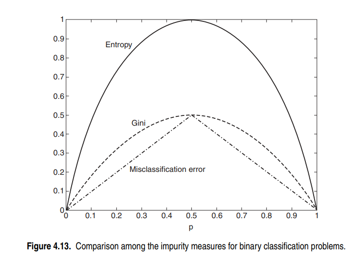
Like the Gini index, a small entropy implies less impurity. The Gini index and entropy are actually quite similar numerically.
You can specify that entropy rather than the Gini index be used in sklearn with sklearn.tree.DecisionTreeClassifier(criterion = 'entropy'). Note that using entropy means sklearn is not technically using CART. This is a technical detail that rarely matters. In practice, we prune and use random forests. If we’re applying random forests, the exact algorithm applied matters doesn’t really make a difference.
Information Gain
Introduction to Data Mining by Steinbach describes information gain well.
Comparing Impurity Measures
Bagging, Random Forests, and Boosting
Bagging, random forests, and boosting uses many decision trees as building blocks to construct a more powerful decision tree.
Bagging (Bootstrap AGGregating)
To understand bagging, we need to know what it means to bootstrap data. To bootstrap data is to resample with replacement from the original, initial same multiple times and to use each resample, bootstramped sample, to compute a statistic. We can gain insight from the computed statistics of our bootstrapped samples. It can be applied to many contexts, not just decision trees. Knowing where the term bootstrap comes from may help us remember its definition. It comes from the idiom “to pull yourself up by your bootstraps” meaning to help or save yourself without help from others. Bootstrapping gleans insight using sample we already have and not by obtaining more samples.
Bagging is also not unique to decision trees. Bagging is just particularly effective with decision trees. Bootstrap aggegation or bagging is a technique where we bootstrap the data, ie resample the data and then create a predictive model from each bootstrapped sample, and then aggregate all the predictive models, using whatever method such as averaging for regression or simple voting for classification. It reduces variance in prediction models.
Random Forests
From Introduction to to Statistical Learning 7th edition, “Random forests provide an improvement over bagged trees by way of a small tweak that decorrelates the trees. As in bagging, we build a number of decision trees on bootstrapped training samples. But when building these decision trees, each time a split in a tree is considered, a random sample of m predictors is chosen as split candidates from the full set of p predictors. The split is allowed to use only one of those m predictors. A fresh sample of m predictors is taken at each split, and typically we choose m ≈ sqrt(p) where p is the number of predictors, also called attributes or features.”
By randomly choosing which predictors to split at in each decision tree, we decorrelate the trees. With bagging alone, we will get many trees that generally split the same way; the decision trees are correlated. Random forests uses decorrelated trees.
Example of Random Forest
The description above is very abstract. Assistant Professor Josh Starmer does a very good job of walking through how to build a random forests with a toy dataset. He uses a classification example and aggregates the data using a simple majority voting system. Remember that there are many ways you can aggregate the data in bagging.