
Market Segmentation Using Customer Data 02 Hunting For Outliers
library(mlbench); library(ggplot2); library(GGally); library(reshape2) # melt fn
source('../src/load_data.r')
Hunting for Outliers using Tukey’s Method
Tukey’s Method
Using Tukey’s Method, outliers are defined as values < $Q_{1} - 1.5IQR$ and values > $Q_{3} + 1.5IQR$ where IQR is the interquartile range.
$IQR = Q_{3} - Q{1}$
where $Q_{1}$ is the value in the dataset >= 25% of the values and <=75% of the values in the datset, $Q_{2}$ is the value >= 50% of the values and <= the rest of the values, and so forth.
options(repr.plot.width = 10, repr.plot.height = 2)

q <- quantile(wholesale_data$Detergents_Paper)
iqr <- q['75%'] - q['25%']
q[['Tukey floor']] <- q['25%'] - 1.5*iqr
q[['Tukey ceiling']] <- q['75%'] + 1.5* iqr

horiz_boxplot <- ggplot(wholesale_data, aes(x = 0, y = Detergents_Paper)) +
                    geom_boxplot(outlier.alpha = 0, size = 1) +
                    coord_flip(ylim = c(-5500, 10000))

points <- geom_jitter(width = 0.1, alpha = 0.1)

labels <- annotate(geom = 'text', y = q, x = c(0.25, -0.25, 0.25, 0.25, -0.25, 0.25, 0.25),
                  label = names(q), check_overlap = FALSE, color = 'darkred')

tukey_window <- annotate(geom = 'line', y = c(q['Tukey floor'], q['Tukey ceiling']),
                         x = 0, size = 20, color = 'darkblue', alpha = 0.5)
text_in_window <- annotate(geom = 'text', x = 0, y = q['50%'],
                           color = 'white',
                           label = 'values not in this range [Q1 - 1.5*IQR, Q3 + 1.5*IQR] are considered outliers')

blank_background <- theme(panel.background = element_blank(),
                          axis.line = element_blank(),
                          axis.ticks = element_blank(),
                          axis.text = element_blank(),
                          axis.title.x = element_blank(),
                          axis.title.y = element_blank())

tukey_graphic <- horiz_boxplot + points + labels + tukey_window + text_in_window + blank_background
print(tukey_graphic)

Changing Size of ‘Tukey Window’
Let’s call the range of values not considered outliers under Tukey’s method, Tukey’s windows for simplicity. It’s not a technical term. We will widen Tukey’s window by changing the factor from 1.5 to 4 because this dataset contains many outliers. There is a large spread so it would be more useful to consider the values on the more extreme ends.
# TODO: ADD display_outliers() to handy_fns or source
display_outliers <- function(feature, param = 4, df = wholesale_data) {
    feature_vec =  as.vector(wholesale_data[[feature]])
    Q1 <- quantile(feature_vec, .25)
    Q3 <- quantile(feature_vec, .75)
    tukey_window <- param*(Q3-Q1)

    # less_than_Q1 & greater_than_Q3 are masks, meaning they're vectors whose
    # elements are booleans
    less_than_Q1 <- wholesale_data[[feature]] < Q1 - tukey_window
    greater_than_Q3 <- wholesale_data[[feature]] > Q3 + tukey_window
    tukey_mask <- (less_than_Q1 | greater_than_Q3)
    outliers <- wholesale_data[tukey_mask,]
    return(outliers)
}
num_df <- Filter(is.numeric, wholesale_data)
outlier_dfs <- sapply(X = colnames(num_df), FUN = display_outliers, simplify = FALSE)
It is nice to be able to see the data frames filtered for outliers, but it’s very granular. Let’s get a count of the number of outliers for each feature.
count_outliers <- function(feature) {
    outlier_count <- dim(display_outliers(feature))[1]
    return(outlier_count)
}

sapply(colnames(Filter(is.numeric, wholesale_data)), count_outliers)
<dl class=dl-horizontal> <dt>Fresh</dt> <dd>2</dd> <dt>Milk</dt> <dd>7</dd> <dt>Grocery</dt> <dd>5</dd> <dt>Frozen</dt> <dd>12</dd> <dt>Detergents_Paper</dt> <dd>9</dd> <dt>Deli</dt> <dd>6</dd> </dl>
## sapply() is difficult because rownames() returns a vector and sapply does not append vectors to return a vector
## it will return a list which messes up following code

raw_outliers <- c()
for (feat in outlier_dfs) {
    ndx <- c(row.names(feat))
    raw_outliers <- c(raw_outliers, ndx)
}

freq_outliers <- as.data.frame(table(raw_outliers))
freq_outliers[freq_outliers$Freq > 1,]
| <th scope=col>raw_outliers</th><th scope=col>Freq</th> | |
|---|---|
| 126 | 2 |
| 182 | 3 |
| 184 | 3 |
| 24 | 2 |
| 334 | 2 |
| 48 | 3 |
| 62 | 3 |
| 66 | 2 |
| 86 | 3 |
| 87 | 2 |
wholesale_data['outlier_for'] <- rownames(wholesale_data) %in% raw_outliers
outliers_many_feats <- freq_outliers[freq_outliers$Freq > 1,]$raw_outliers
many_feats <- rownames(wholesale_data) %in% outliers_many_feats
wholesale_data$outlier_for[many_feats] <- 'many_feats'
wholesale_data$outlier_for[wholesale_data$outlier_for == TRUE] <- 'one_feat'
wholesale_data$outlier_for[wholesale_data$outlier_for == FALSE] <- 'zero'
head(wholesale_data)
| Retail | Other | 12669 | 9656 | 7561 | 214 | 2674 | 1338 | zero |
| Retail | Other | 7057 | 9810 | 9568 | 1762 | 3293 | 1776 | zero |
| Retail | Other | 6353 | 8808 | 7684 | 2405 | 3516 | 7844 | one_feat |
| Horeca | Other | 13265 | 1196 | 4221 | 6404 | 507 | 1788 | zero |
| Retail | Other | 22615 | 5410 | 7198 | 3915 | 1777 | 5185 | zero |
| Retail | Other | 9413 | 8259 | 5126 | 666 | 1795 | 1451 | zero |
From R Documentation:
ggpairs(data, mapping = NULL, columns = 1:ncol(data), title = NULL,
  upper = list(continuous = "cor", combo = "box_no_facet", discrete =
  "facetbar", na = "na"), lower = list(continuous = "points", combo =
  "facethist", discrete = "facetbar", na = "na"), diag = list(continuous =
  "densityDiag", discrete = "barDiag", na = "naDiag"), params = NULL, ...,
  xlab = NULL, ylab = NULL, axisLabels = c("show", "internal", "none"),
  columnLabels = colnames(data[columns]), labeller = "label_value",
  switch = NULL, showStrips = NULL, legend = NULL,
  cardinality_threshold = 15, legends = stop("deprecated"))
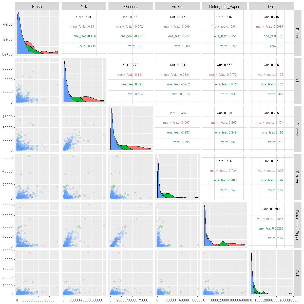
options(repr.plot.width = 10, repr.plot.height = 10)

pairplot_products <- function(data) {
    ggpairs(data = data,
            columns = c('Fresh','Milk', 'Grocery', 'Frozen', 'Detergents_Paper', 'Deli'),
            mapping = aes(color = outlier_for),
            upper = list(continuous = wrap(ggally_cor, size = 2.5, alignPercent = 0.8)),
            lower = list(continuous = wrap(ggally_points, alpha = 0.2)),
           )
}
pairplot_products(wholesale_data)
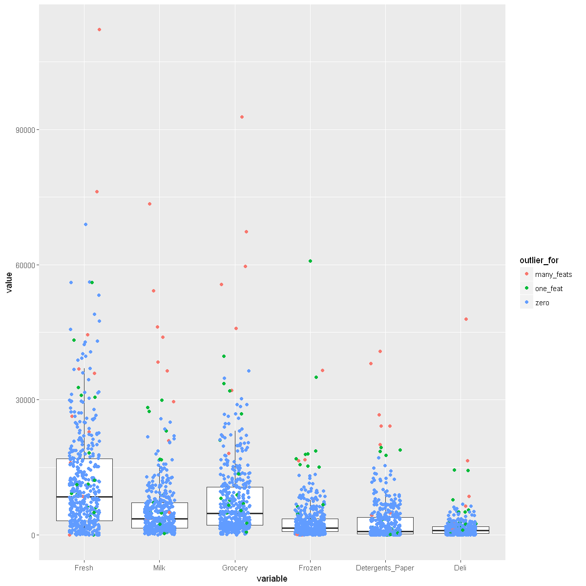
boxplot_product <- function(data) {
    ggplot(melt(data), aes(x = variable, y = value)) +
        geom_boxplot(outlier.alpha = 0) +
        geom_jitter(width = .2, aes(color = outlier_for))
}

boxplot_product(wholesale_data)
Using Channel, Region, outlier_for as id variables
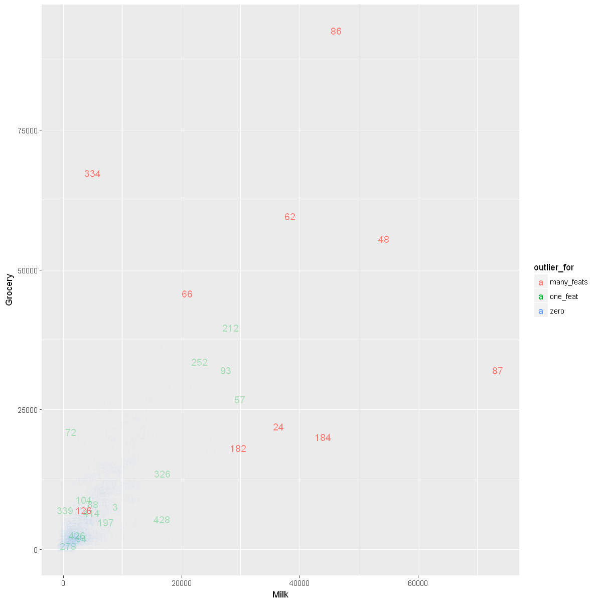
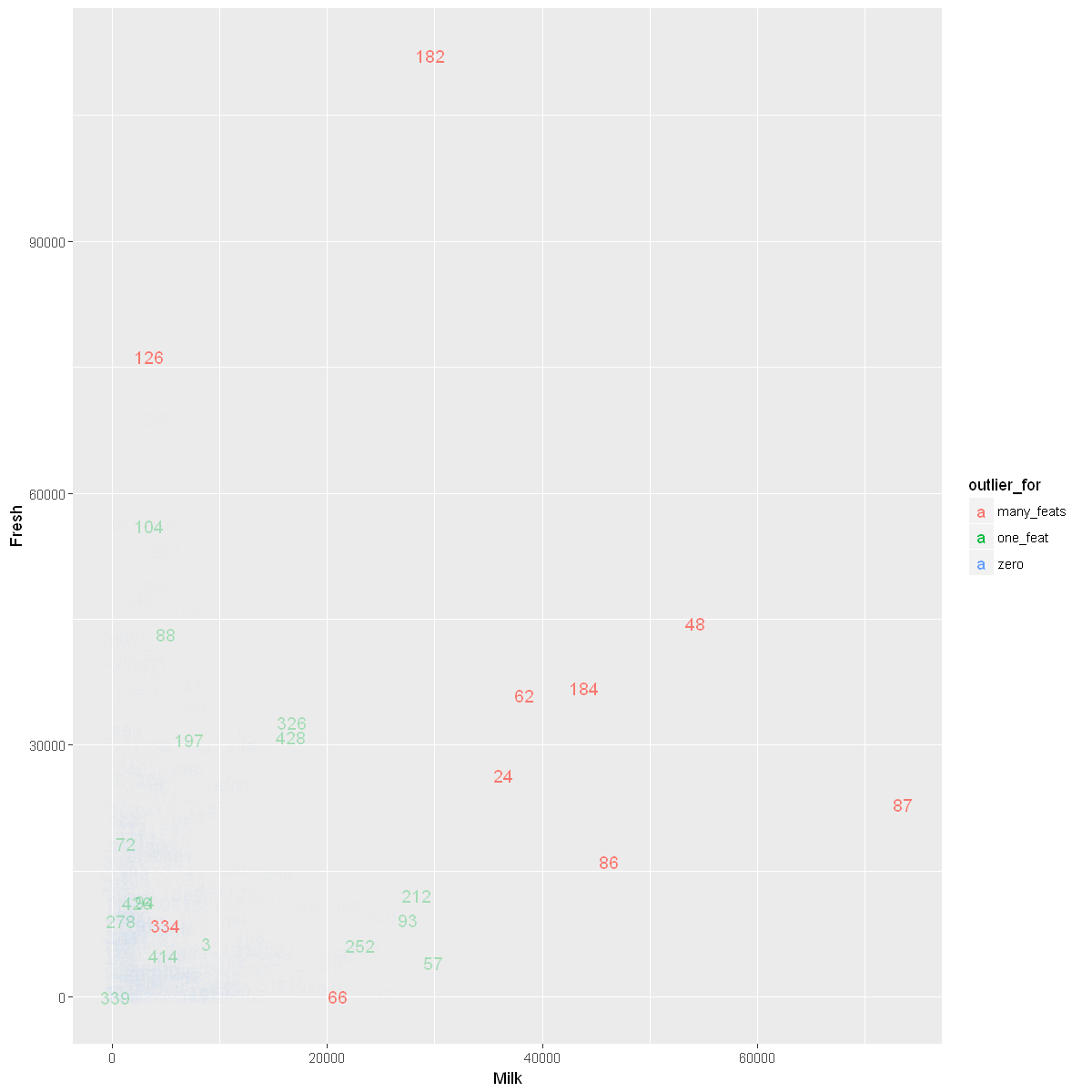
show_outliers_in_scatter <- function(xFeat, yFeat) {
    ggplot(wholesale_data, aes_string(x = substitute(xFeat), y = substitute(yFeat), color = 'outlier_for',
                                alpha = 'outlier_for')) +
    geom_text(check_overlap = FALSE, size = 4, aes(label = rownames(wholesale_data))) +
    scale_alpha_manual(guide = 'none', values = list(zero = 0.02, one_feat = 0.3, many_feats = 1))
}

show_outliers_in_scatter(Milk, Grocery)
show_outliers_in_scatter(Milk, Fresh)
show_outliers_in_scatter(Frozen, Grocery)
show_outliers_in_scatter(Deli, Detergents_Paper)
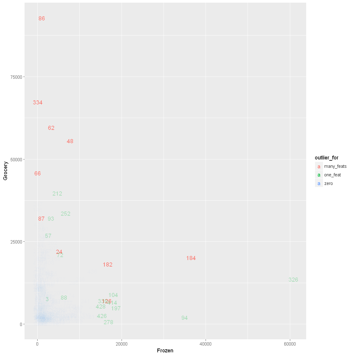
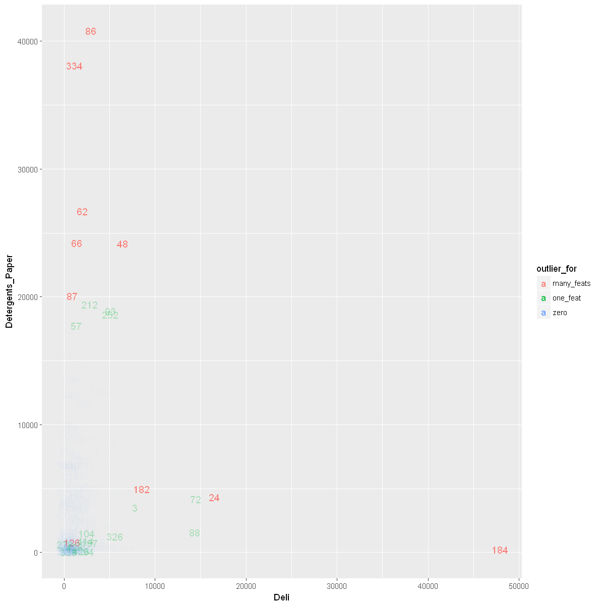
Visualizing Data Without Outliers That Are Outliers for Multiple Features
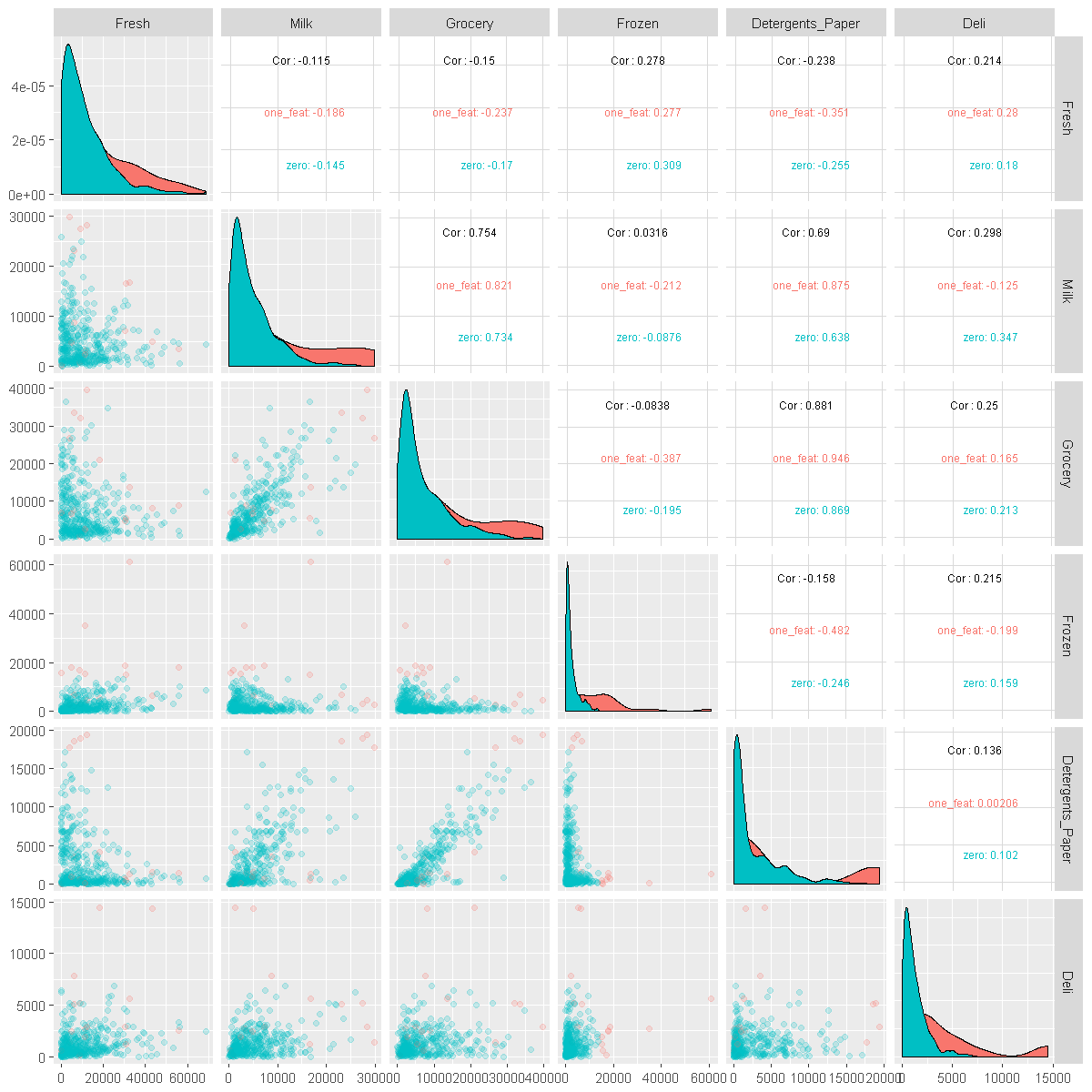
Let’s first see how many observations are outliers for multiple features.
dim(wholesale_data[wholesale_data$outlier_for != 'many_feats',])
<ol class=list-inline> <li>430</li> <li>9</li> </ol>
pairplot_products(wholesale_data[wholesale_data$outlier_for != 'many_feats',])
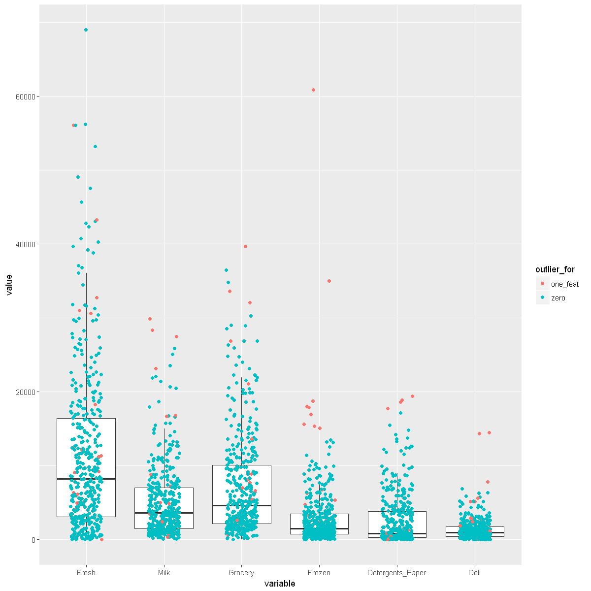
boxplot_product(wholesale_data[wholesale_data$outlier_for != 'many_feats',])
Using Channel, Region, outlier_for as id variables
Verdict: Not Quite Removing Outliers
Usually, we would remove some outliers but there appears that outliers for many features are also the most extreme outliers within each feature. In practice, these outliers are significant because they represent customers that bring in a lot of business. We would be wise to not ignore them when analyzing our customers. However, while doing cluster modeling, these outliers will just add noise to our analysis of most of our customers. Thus, we will not consider these outliers that are outliers for many features in our clustering analysis.
wholesale_data <- wholesale_data[wholesale_data$outlier_for != 'many_feats',]
clean_wholesale <- subset(wholesale_data, select = -c(outlier_for))
write.csv(clean_wholesale, file = '../data/clean_wholesale.csv')