
Optimizing Sample Size in AB Tests (edited 2021-01-03)
Definition of A/B Testing
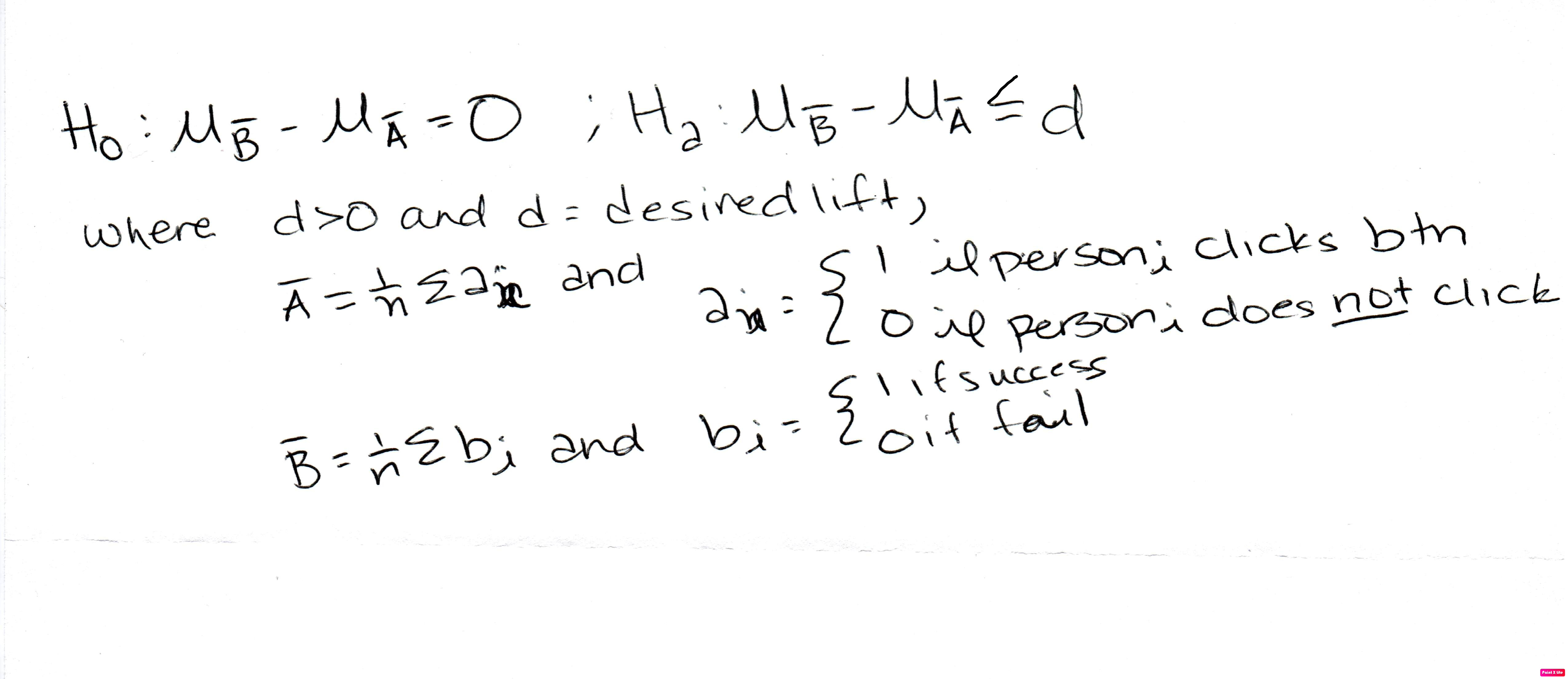
An A/B test is a hypothesis test where the null hypothesis is that variant A and variant B of a feature have the
same performance on a given metric. For example, the null hypothesis can be that users are just as likely to click
on a “sign up” button that is the current button color red as a green button. In that case, the number of clicks is
the performance metric, a red button is variant A and a green button is variant B.
The alternative hypothesis is that the green button performs better by some number of clicks,
we’ll call this the desired lift.
Why do we care about sample size?
Intuitively, larger sample sizes are more convincing. The more members of a group that have some feature or behavior, the more we can confidently infer that the rest of the group have the same feature or behavior. The more we test the performance of variant B, a green button, the more we can be certain of its performance with more users.
Mathematically modeling proves our intuition correct and let’s us be more precise. There are business constraints on sample size. A business risks user engagement each time it presents a user with a new green button rather than their tried and tested red button.
With What Sample Size Would You Be Comfortable?
Confusion Matrix
To answer that question we need to know acceptable thresholds for statistical power, significance level α, and beta ß. These three values are described in confusion matrices.
Confusion Matrix
| actual ↓ predicted → | True | False |
|---|---|---|
| True | statistical power | false negative; Type I error; ß |
| False | false positive; Type II error; α; p-level |
How does sample size affect statistical power, significance level α, and Type 1 error ß?
 “bernoulli-to-binomial-to-approximating-normal”)
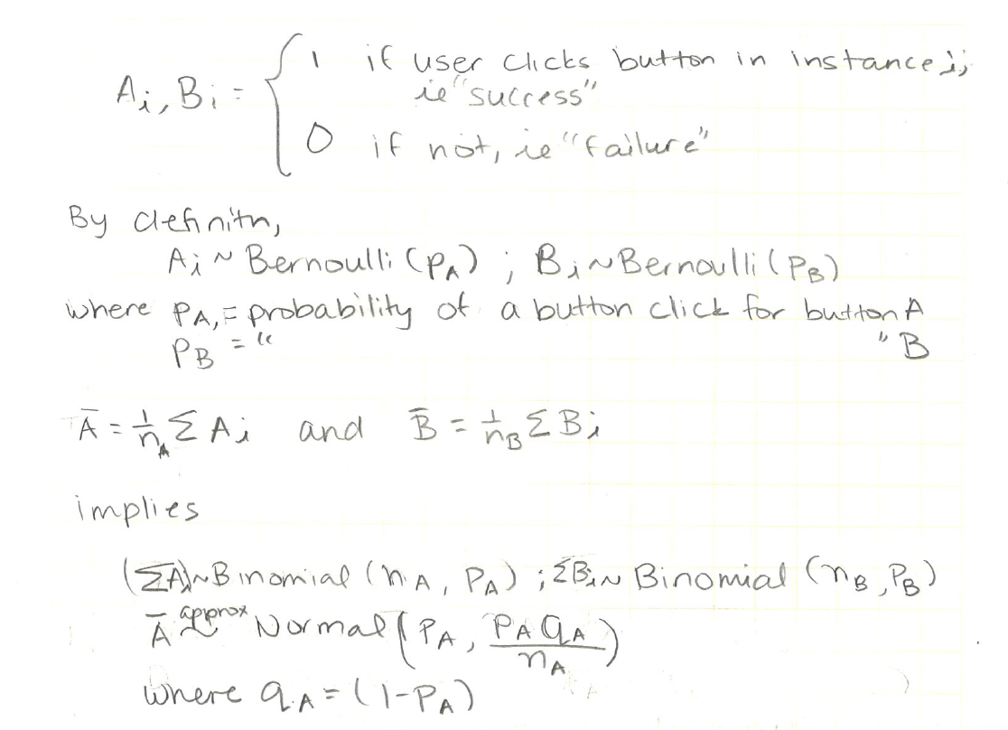
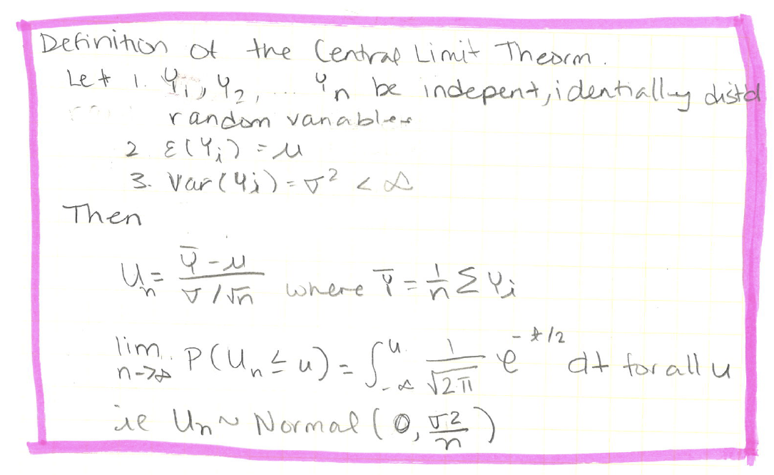
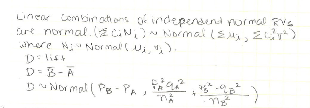
According to the central limit theorem, and are asymptotically nomrally distributed for large n. Empirically, we have found n > 30 to be closely normal. our goal is to minimize sample size, but exact calculations are cumbersome. Approximating will still illustrate key points that apply to small samples too. We will see that is better to first approximate sample sizes that we are comfortable and if they are small, less than 30, then it may be worthwhile to make exact calculations.
Graphing statistical power, , and with R
Statistical power is the green area. It is the probability of rejecting the null hypothesis when the alternative hypothesis is true. It is the probability of a true positive.
Significance level, also called the alpha level, is the pink area. It is the probability of rejecting the null hypothesis when the null hypothesis is true. It is the probability of a false positive, a Type I error.
Beta is the blue area. It is the probability of not rejecting the null hypothesis when the alternative hypothesis is true. It is the probability of a false positive, a Type II error.
library(ggplot2); library(GGally)
shade_norm <- function(c, xlimits, mean_ = 0) {
    stat_function(fun = dnorm, args = list(mean = mean_),
              xlim = xlimits, geom = 'area',
              fill = c, alpha = 0.5,
              color = c, size = 1)
}

v_line <- function(x_intercept) {
    geom_vline(xintercept = x_intercept,
               size = 0.7, linetype='dashed', alpha = 0.5)
}
options(repr.plot.height = 3, repr.plot.width = 6)

label_values = list('α' = 1.65, 'd' = 2.5, 'µ_H0 = 0' = 0)
z_df <- data.frame(z = seq(-3.5, 3.5, 0.01))

#alpha = 0.05; this a right-tailed H test
z_a = label_values[['a']]
z_d = label_values[['d']]

alpha <- shade_norm('pink', c(z_a, 3.2))
power <- shade_norm('green', c(z_a, 6.5), z_d)
beta <- shade_norm('light blue', c(z_a, -1.2), z_d)

H_0 <- stat_function(fun = dnorm)
H_a <- stat_function(fun = dnorm, args = list(mean = z_d))
y_axis <- geom_vline(xintercept = 0, size = 0.7)

gg <- ggplot(z_df, aes(z)) +
    H_0 + H_a + y_axis +
    beta + power + alpha +
    scale_x_continuous(breaks = unlist(label_values),
                       label = names(label_values),
                       limits = c(-3.5, 6.5)) +
    make_vlines(label_values) +
    ylab('density')
print(gg)
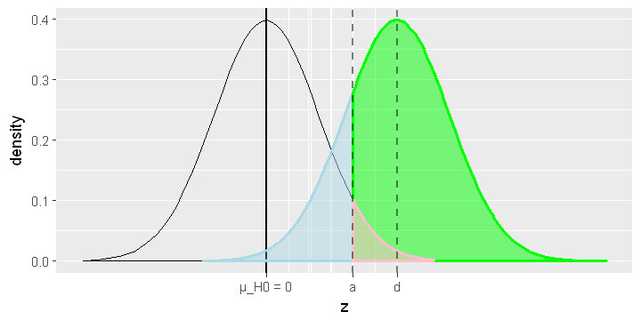
As we can see from the chart above, we want to minimize α and ß. Recall that according to the Central Limit Theorem, as we increase the sample size, the two curves narrow. Thus, as we increase the sample size, alpha and beta decrease.
What is the minimum sample if we want statistical power, ß, alpha level α, and desired life d?
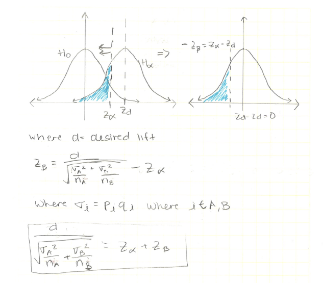
We can see that the greate the statistical power and the lower the probability of Type I and Type II errors, ie α and ß; the larger our sample size needs to be.
Small Sizes
If our approximate calculations lead us to conclude that smaller sample sizes are sufficient, it is worthwhile to calculate without approximating to nomral. However, as we can see, those are rare cases where we are quite liberal with statistical power, α, and ß.
Stray Observation
Consider the case where variant A, the red button, is in production and, thus, already has a very large sample size.
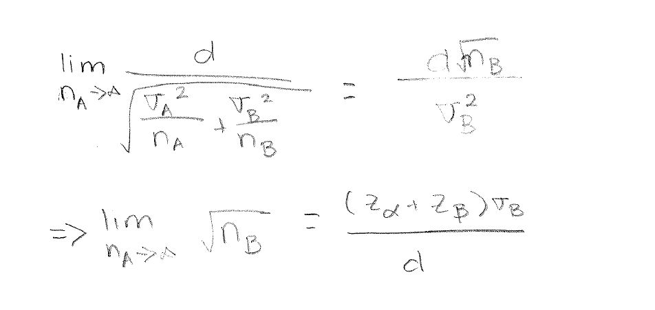
This is equivalent to a single-variable test where
