Spooky Author Identification
This is how I tackled the Spooky Author Identification challenge on Kaggle.
import warnings
warnings.filterwarnings('ignore')
import pandas as pd

from sklearn.model_selection import train_test_split,\
                                        GridSearchCV,\
                                        ShuffleSplit

from sklearn.feature_extraction.text import ENGLISH_STOP_WORDS,\
                                                TfidfVectorizer

from sklearn.svm import SVC
from sklearn.linear_model import LogisticRegression
from sklearn.naive_bayes import MultinomialNB
from sklearn.metrics import log_loss

from matplotlib_venn import venn3
import seaborn as sns

from nltk import word_tokenize
from nltk.stem.porter import PorterStemmer
from nltk.stem import WordNetLemmatizer
import nltk
nltk.download('wordnet')

from collections import namedtuple
from itertools import product
Load Data
train_df = pd.read_csv('data/train.csv')
test_df = pd.read_csv('data/test.csv')

y = train_df.author
x = train_df.text

random_seed = 0

x_train, x_valid, y_train, y_valid = train_test_split(x, y,
                                                      random_state=random_seed)
Basic EDA
Distribution of Target Variable
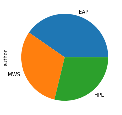
The distribution of the target variable, author, is homogenous. This informs how I create my models. I will not need to stratify my bootstrapped data and can be less picky about which model to use. Some models perform better than others on imbalanced data.
# distribution of target variable is homogenous
# means I will not need to stratify my bootstrapped data
%matplotlib inline
y.value_counts().plot('pie')
<matplotlib.axes._subplots.AxesSubplot at 0x2220724dc18>

Eyeballing Data
I like to actually look at my data before doing anything, in the hopes that I can find any patterns myself and not rely solely on models. Nothing is really jumping out at me. I will just proceed as usual.
def print_sample(sub_df):
    writing_samples = sub_df.text\
                                .sample(n=5, random_state=random_seed)\
                                .str.cat()
    print(sub_df.name)
    print(writing_samples)
    print()
train_df.groupby('author').apply(print_sample)
EAP
Leaving this drawer, as well as cupboard No. open, Maelzel now unlocks door No. , and door No. , which are discovered to be folding doors, opening into one and the same compartment.He seems to have been very much averse to permitting the relatives to see the body."I want the damages at a thousand, but he says that for so simple a knock down we can't lay them at more than five hundred.Miss Tabitha Turnip propagated that report through sheer envy.The tints of the green carpet faded; and, one by one, the ruby red asphodels withered away; and there sprang up, in place of them, ten by ten, dark, eye like violets, that writhed uneasily and were ever encumbered with dew.
HPL
I was sorry I had put out the light, yet was too tired to rise and turn it on again.The borders of the space were entirely of brick, and there seemed little doubt but that he could shortly chisel away enough to allow his body to pass.Then one night as I listened at the door I heard the shrieking viol swell into a chaotic babel of sound; a pandemonium which would have led me to doubt my own shaking sanity had there not come from behind that barred portal a piteous proof that the horror was real the awful, inarticulate cry which only a mute can utter, and which rises only in moments of the most terrible fear or anguish.I shiver as I speak of them, and dare not be explicit; though I will say that my friend once wrote on paper a wish which he dared not utter with his tongue, and which made me burn the paper and look affrightedly out of the window at the spangled night sky.But for one thing Old Bugs would have been an ideal slave to the establishment and that one thing was his conduct when young men were introduced for their first drink.
MWS
Then, in endeavouring to do violence to my own disposition, I made all worse than before.The pretty Miss Mansfield has already received the congratulatory visits on her approaching marriage with a young Englishman, John Melbourne, Esq.The Earl of Windsor became a volunteer under his friend.A truce was concluded between the Greeks and Turks."I come to you," he said, "only half assured that you will assist me in my project, but resolved to go through with it, whether you concur with me or not.
Overlap of Words Used
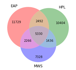
The more distnct each author is in their writing, the easier it will be to determine the authorship of a sentence. The venn diagram below shows that each author does have many words not used by other authors.
def accept_series_arg(word_tokenize_fn):
    def inner(arg):
        if isinstance(arg, pd.Series):
            text = arg.str.cat()
            return word_tokenize_fn(text)
        else:
            return word_tokenize_fn(arg)
    return inner
word_tokenize = accept_series_arg(word_tokenize)
author_tokens = {a: set(word_tokenize(train_df.text[train_df.author==a]))
                                             for a in train_df.author.unique()}
venn3(author_tokens.values(), author_tokens.keys())
<matplotlib_venn._common.VennDiagram at 0x22207829048>

English Stop Words
A challenge in text classification is that there are many, many features. This requires a lot of computing and puts more strain on our models. Thus, feature engineering can be especially helpful.
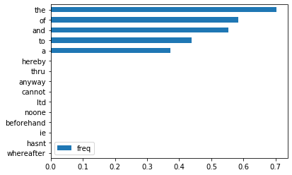
It could be useful to drop words that appear so rarely or frequently in our corpus, such that they do not inform our model. To help me determine how to do that, I looked at the document frequency of words in Sci-Kit Learn’s list of English stop words in this corpus.
Also, I suspect that Sci-Kit Learn’s stop words may be more for modern times than the authors in our dataset. If so, with more time, I would consider modifying that list.
def get_doc_freq(docs, tokens):
    counts = {t: 0 for t in tokens}

    def count_token_freq(text):
        text = word_tokenize(text)
        for k in counts:
            if k in text:
                counts[k] += 1

    for text in docs:
        count_token_freq(text)

    counts_df = pd.DataFrame(counts.values(),
                             index = counts.keys(),
                             columns=['freq']).sort_values(by='freq')
    counts_df.freq = counts_df.freq/len(docs)
    return counts_df


doc_freq = get_doc_freq(train_df.text, ENGLISH_STOP_WORDS)
pd.concat([doc_freq.head(10), doc_freq.tail(5)]).plot(kind='barh')
<matplotlib.axes._subplots.AxesSubplot at 0x22207852f60>

Processing
Tokens and Stop Words
I considered stemming and lemmatizing words. I ultimately decided on lemmatizing words. Also, I’m filtering out stop words in the tokenizer to be passed into TfidVectorizer instead of passing stop words into TfidVectorizer to filter. This is because TfidVectorizer tokenizes and then drops any tokens in the list of stop words. The problem is that sometimes, tokening a stop word changes it, so TfidVectorizer does not drop it.
def tokenize(text, base='lemma'):
    if base == 'stem':
        normalizer = PorterStemmer().stem
    elif base == 'lemma':
        normalizer = WordNetLemmatizer().lemmatize
    else:
        raise ValueError("base can only be 'stem', or 'lemma'")
    tokens = [normalizer(t) for t in word_tokenize(text)\
                                if t not in ENGLISH_STOP_WORDS]
    return tokens
Modeling
Hypertuning Parameters
I will iterate through different parameters to determine the best parameters.
def get_modelcv(model):
    def inner(param_grid):
        grid = GridSearchCV(model(),
                            param_grid=param_grid,
                            cv=ShuffleSplit(n_splits=5,
                                            test_size=0.20,
                                            random_state=random_seed))
        grid.fit(X_train_tfidf, y_train)

        tuned_model = model(**grid.best_params_)
        tuned_model.fit(X_train_tfidf, y_train)
        return tuned_model
    return inner
tfidf_vectors = namedtuple('tfidf_vectors', ['train', 'valid'])
def process_text(min_df, max_df):
    tfidf_vectorizer = TfidfVectorizer(tokenizer=tokenize,
                                       min_df = min_df,
                                       max_df = max_df,
                                       stop_words=None,
                                       smooth_idf=True)
    tfidf_vectorizer.fit(x_train)
    X_train_tfidf = tfidf_vectorizer.transform(x_train)
    X_valid_tfidf = tfidf_vectorizer.transform(x_valid)
    return tfidf_vectors(X_train_tfidf, X_valid_tfidf)
Models
Logistic regression, naive bayes, and support vector machine are popular models for text classification because they perform relatively well on small data. This dataset of almost 20,000 observations is small because the number of observations is small relative to the number of features. Text data has many, many features.
train_df.shape
(19579, 3)
Parameters
I was initially planning on iterating through more parameters, but that took too long, especially for SVC. Logistic Regression did not take as long so I will try different “penalties”, loss functions.
For Naive Bayes, I do not need to tune for alpha, the additive (Laplace/Lidstone) smoothing parameter.
where is the total number of documents in the corpus and document frequency.
I already set tfidf_vectorizer parameter smooth_idf=True which adds “one to document frequencies, as if an extra document was seen containing every term in the collection exactly once. Prevents zero divisions.”. Thus,
Also, the larger we set α to be, the more we will warp our dataset and make our models perform worse.
At most, Adding α will change the proportions and give more weight to terms with small TFIDFs.
model_to_param_grid = {LogisticRegression: {'penalty':('l2','l1')},
                       MultinomialNB: {'alpha':[0]},
                       SVC: {'C': [1],
                             'gamma': [2**-1],
                             'kernel': ['rbf'],
                             'probability': [True]}}
record = namedtuple('clf', ['clf', 'score', 'min_df', 'max_df'])
min_dfs = [4, 16]
max_dfs = [0.7, 0.99]
tuned_models = list()
for mn, mx in product(min_dfs, max_dfs):
    X_train_tfidf, X_valid_tfidf = process_text(mn, mx)
    for m, pg in model_to_param_grid.items():
        classifier = get_modelcv(m)(pg)
        probas = classifier.predict_proba(X_valid_tfidf)
        score = log_loss(y_valid, probas)
        print(record(classifier, score, mn, mx))
        tuned_models.append(record(classifier, score, mn, mx))
clf(clf=LogisticRegression(C=1.0, class_weight=None, dual=False, fit_intercept=True,
                   intercept_scaling=1, l1_ratio=None, max_iter=100,
                   multi_class='warn', n_jobs=None, penalty='l2',
                   random_state=None, solver='warn', tol=0.0001, verbose=0,
                   warm_start=False), score=0.6165282240393588, min_df=4, max_df=0.7)
clf(clf=MultinomialNB(alpha=0, class_prior=None, fit_prior=True), score=0.9642711984140351, min_df=4, max_df=0.7)
clf(clf=SVC(C=1, cache_size=200, class_weight=None, coef0=0.0,
    decision_function_shape='ovr', degree=3, gamma=0.5, kernel='rbf',
    max_iter=-1, probability=True, random_state=None, shrinking=True, tol=0.001,
    verbose=False), score=0.5133220283089204, min_df=4, max_df=0.7)
clf(clf=LogisticRegression(C=1.0, class_weight=None, dual=False, fit_intercept=True,
                   intercept_scaling=1, l1_ratio=None, max_iter=100,
                   multi_class='warn', n_jobs=None, penalty='l2',
                   random_state=None, solver='warn', tol=0.0001, verbose=0,
                   warm_start=False), score=0.6118237123501002, min_df=4, max_df=0.99)
clf(clf=MultinomialNB(alpha=0, class_prior=None, fit_prior=True), score=0.9559776177898892, min_df=4, max_df=0.99)
clf(clf=SVC(C=1, cache_size=200, class_weight=None, coef0=0.0,
    decision_function_shape='ovr', degree=3, gamma=0.5, kernel='rbf',
    max_iter=-1, probability=True, random_state=None, shrinking=True, tol=0.001,
    verbose=False), score=0.5068561285275058, min_df=4, max_df=0.99)
clf(clf=LogisticRegression(C=1.0, class_weight=None, dual=False, fit_intercept=True,
                   intercept_scaling=1, l1_ratio=None, max_iter=100,
                   multi_class='warn', n_jobs=None, penalty='l2',
                   random_state=None, solver='warn', tol=0.0001, verbose=0,
                   warm_start=False), score=0.6442031955034971, min_df=16, max_df=0.7)
clf(clf=MultinomialNB(alpha=0, class_prior=None, fit_prior=True), score=0.6563940208150089, min_df=16, max_df=0.7)
clf(clf=SVC(C=1, cache_size=200, class_weight=None, coef0=0.0,
    decision_function_shape='ovr', degree=3, gamma=0.5, kernel='rbf',
    max_iter=-1, probability=True, random_state=None, shrinking=True, tol=0.001,
    verbose=False), score=0.6033604930633173, min_df=16, max_df=0.7)
clf(clf=LogisticRegression(C=1.0, class_weight=None, dual=False, fit_intercept=True,
                   intercept_scaling=1, l1_ratio=None, max_iter=100,
                   multi_class='warn', n_jobs=None, penalty='l2',
                   random_state=None, solver='warn', tol=0.0001, verbose=0,
                   warm_start=False), score=0.6408116465101706, min_df=16, max_df=0.99)
clf(clf=MultinomialNB(alpha=0, class_prior=None, fit_prior=True), score=0.6536898470534854, min_df=16, max_df=0.99)
clf(clf=SVC(C=1, cache_size=200, class_weight=None, coef0=0.0,
    decision_function_shape='ovr', degree=3, gamma=0.5, kernel='rbf',
    max_iter=-1, probability=True, random_state=None, shrinking=True, tol=0.001,
    verbose=False), score=0.5955775184613233, min_df=16, max_df=0.99)
Results
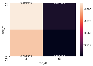
It appears that not filtering out a lot of features, ie setting the document frequency floor at 4 documents and ceiling at 99% of documents, and using support vector machines is best.
I’m not surprised that support vector machines perform best, although they do require more computational power.
I was not expecting logistic regression to perform better than naive bayes. Naive bayes tend to perform better on smaller data sets (Logistic regression will overfit.) and logistic regression on larger data sets (naive bayes will underfit), but that’s not a hard rule.
tuned_models = pd.DataFrame(tuned_models)
sns.heatmap(tuned_models\
                .groupby(['min_df', 'max_df'])\
                .mean()\
                .reset_index()\
                .pivot(index='max_df', columns='min_df', values='score'),
            annot=True, fmt='f')
<matplotlib.axes._subplots.AxesSubplot at 0x222085596d8>

tuned_models.sort_values('score').style.bar(subset='score')
| clf | score | min_df | max_df | |
|---|---|---|---|---|
| 5 | SVC(C=1, cache_size=200, class_weight=None, coef0=0.0, decision_function_shape='ovr', degree=3, gamma=0.5, kernel='rbf', max_iter=-1, probability=True, random_state=None, shrinking=True, tol=0.001, verbose=False) | 0.506856 | 4 | 0.99 |
| 2 | SVC(C=1, cache_size=200, class_weight=None, coef0=0.0, decision_function_shape='ovr', degree=3, gamma=0.5, kernel='rbf', max_iter=-1, probability=True, random_state=None, shrinking=True, tol=0.001, verbose=False) | 0.513322 | 4 | 0.7 |
| 11 | SVC(C=1, cache_size=200, class_weight=None, coef0=0.0, decision_function_shape='ovr', degree=3, gamma=0.5, kernel='rbf', max_iter=-1, probability=True, random_state=None, shrinking=True, tol=0.001, verbose=False) | 0.595578 | 16 | 0.99 |
| 8 | SVC(C=1, cache_size=200, class_weight=None, coef0=0.0, decision_function_shape='ovr', degree=3, gamma=0.5, kernel='rbf', max_iter=-1, probability=True, random_state=None, shrinking=True, tol=0.001, verbose=False) | 0.60336 | 16 | 0.7 |
| 3 | LogisticRegression(C=1.0, class_weight=None, dual=False, fit_intercept=True, intercept_scaling=1, l1_ratio=None, max_iter=100, multi_class='warn', n_jobs=None, penalty='l2', random_state=None, solver='warn', tol=0.0001, verbose=0, warm_start=False) | 0.611824 | 4 | 0.99 |
| 0 | LogisticRegression(C=1.0, class_weight=None, dual=False, fit_intercept=True, intercept_scaling=1, l1_ratio=None, max_iter=100, multi_class='warn', n_jobs=None, penalty='l2', random_state=None, solver='warn', tol=0.0001, verbose=0, warm_start=False) | 0.616528 | 4 | 0.7 |
| 9 | LogisticRegression(C=1.0, class_weight=None, dual=False, fit_intercept=True, intercept_scaling=1, l1_ratio=None, max_iter=100, multi_class='warn', n_jobs=None, penalty='l2', random_state=None, solver='warn', tol=0.0001, verbose=0, warm_start=False) | 0.640812 | 16 | 0.99 |
| 6 | LogisticRegression(C=1.0, class_weight=None, dual=False, fit_intercept=True, intercept_scaling=1, l1_ratio=None, max_iter=100, multi_class='warn', n_jobs=None, penalty='l2', random_state=None, solver='warn', tol=0.0001, verbose=0, warm_start=False) | 0.644203 | 16 | 0.7 |
| 10 | MultinomialNB(alpha=0, class_prior=None, fit_prior=True) | 0.65369 | 16 | 0.99 |
| 7 | MultinomialNB(alpha=0, class_prior=None, fit_prior=True) | 0.656394 | 16 | 0.7 |
| 4 | MultinomialNB(alpha=0, class_prior=None, fit_prior=True) | 0.955978 | 4 | 0.99 |
| 1 | MultinomialNB(alpha=0, class_prior=None, fit_prior=True) | 0.964271 | 4 | 0.7 |
Testing
tfidf_vectorizer = TfidfVectorizer(tokenizer=tokenize,
                                   min_df = 4,
                                   max_df = 0.99,
                                   stop_words=None,
                                   smooth_idf=True)
tfidf_vectorizer.fit(x_train)
TfidfVectorizer(analyzer='word', binary=False, decode_error='strict',
                dtype=<class 'numpy.float64'>, encoding='utf-8',
                input='content', lowercase=True, max_df=0.99, max_features=None,
                min_df=4, ngram_range=(1, 1), norm='l2', preprocessor=None,
                smooth_idf=True, stop_words=None, strip_accents=None,
                sublinear_tf=False, token_pattern='(?u)\\b\\w\\w+\\b',
                tokenizer=<function tokenize at 0x00000222087F20D0>,
                use_idf=True, vocabulary=None)
test_tfidf = tfidf_vectorizer.transform(test_df.text.values)
best_model = tuned_models.sort_values('score').clf.values[0]
probas = best_model.predict_proba(test_tfidf)
# y_train.unique() will be in the right order because it will just be the order that
# each author is listed
submission = pd.DataFrame(probas, index=test_df.id, columns = y.drop_duplicates().sort_values())
submission.to_csv('submission.csv')
Score
I submitted my predicted probabilities for Kaggle to score. My score (log loss is the evaluation metric for this competition) is 0.49077.