Predicting Housing Prices 05 Linear Models My Best Performers
import numpy as np
import pandas as pd
import warnings; warnings.filterwarnings('ignore')
%matplotlib inline
import pickle
from sklearn import linear_model
train = pd.read_pickle('../data/train.p')
Preparing Data for Linear Models
We need to deskew the independent variables to lessen the effects of influential outliers. There are many ways to make skewed data more centered. Taking the log worked best.
NB It is a common misconception that for linear models, the distribution of the independent variables need to be normal. There is no assumption that the distributions need to be normal for linear models to perform well. We do not transform our independent variables to make its distribution more normal. We transform our data for the following reasons:
- To deskew the distribution to minimize the effect of influential outliers.
- To make our independent and dependent variables have a linear relationship. A linear relationship between these two variables is an assumption of the linear model.
def addlogs(res, ls):
    for l in ls:
        log_transforms = pd.Series(np.log(1.01+res[l]), name='log_'+l)
        res = pd.concat((res, log_transforms), axis=1)
    return res

to_log = ['LotFrontage', 'LotArea', 'YearBuilt', 'YearRemodAdd', 'MasVnrArea',
       'BsmtFinSF1', 'BsmtFinSF2', 'BsmtUnfSF', 'TotalBsmtSF', '1stFlrSF',
       '2ndFlrSF', 'LowQualFinSF', 'GrLivArea', 'GarageArea', 'WoodDeckSF',
       'OpenPorchSF', 'EnclosedPorch', 'ThreeSsnPorch', 'ScreenPorch',
       'PoolArea', 'MiscVal', 'SalePrice']
train = addlogs(train, to_log)
test = pd.read_pickle('../data/test.p')
to_log_less_target = to_log = ['LotFrontage', 'LotArea', 'YearBuilt', 'YearRemodAdd', 'MasVnrArea',
       'BsmtFinSF1', 'BsmtFinSF2', 'BsmtUnfSF', 'TotalBsmtSF', '1stFlrSF',
       '2ndFlrSF', 'LowQualFinSF', 'GrLivArea', 'GarageArea', 'WoodDeckSF',
       'OpenPorchSF', 'EnclosedPorch', 'ThreeSsnPorch', 'ScreenPorch',
       'PoolArea', 'MiscVal']
test = addlogs(test, to_log_less_target)
X = train.drop(columns=['log_SalePrice', 'SalePrice'] + to_log )
test = test.drop(columns = to_log)

y = train.log_SalePrice
from sklearn.preprocessing import StandardScaler
rows_test = set(test.index)
rows_train = set(X.index)
rows_test & rows_train
set()
Unsurprisingly, we found that linear models without penalties did not perform well because there is a lot of multicollinearity in this dataset. LASSO and Ridge add penalties and is the easiest way to minimize the damage done by multicollinearity. How LASSO and Ridge do this is in one of my write-ups. The harder option is to drop or combine features to reduce multicollinearity.
dummies = pd.get_dummies(X.append(test), drop_first= True)

X_dummies = dummies.loc[list(rows_train)]
test_dummies = dummies.loc[list(rows_test)]
from sklearn.preprocessing import StandardScaler
scaler = StandardScaler()
X_scaled = scaler.fit_transform(X_dummies)
test_scaled = scaler.transform(test_dummies)
from sklearn.metrics import mean_squared_log_error
from math import e
lassoCV = linear_model.LassoCV()
lassoCV.fit(X_scaled, y)

scr = lassoCV.score(X_scaled, y)
rmsle = np.sqrt(mean_squared_log_error(e**lassoCV.predict(X_scaled), e**y))
print('lassoCV.score = ', scr)
print('rmsle = ', rmsle)
def plot_coef(model, top_n = 10):
    '''
    Plots the magnitude of coefficients
    '''
    cols = X.columns
    coef = model.coef_
    zipped = list(zip(cols, coef))
    zipped.sort(key=lambda x: x[1], reverse = True)
    top_10 = pd.DataFrame(zipped).head(top_n)
    bottom_10 = pd.DataFrame(zipped).tail(top_n)
    return pd.concat([top_10, bottom_10], axis=0).plot.barh(x = 0, y = 1)

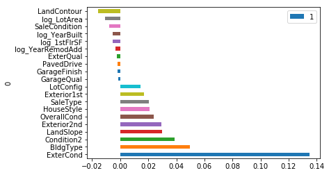
plot_coef(lassoCV)
lassoCV.score =  0.9372230213206038
rmsle =  0.1001291553254421


<matplotlib.axes._subplots.AxesSubplot at 0x27a3f08d080>

submission = pd.DataFrame({'SalePrice': e**lassoCV.predict(test_scaled)},
                         index = test.index)
submission.to_csv('ames-submission-5.csv')
log transforming the data helps

ridgeCV = linear_model.RidgeCV()
ridgeCV.fit(X_scaled, y)
scr = ridgeCV.score(X_scaled, y)
rmsle = np.sqrt(mean_squared_log_error(e**ridgeCV.predict(X_scaled), e**y))
print('ridgeCV.score = ', scr)
print('rmsle = ', rmsle)

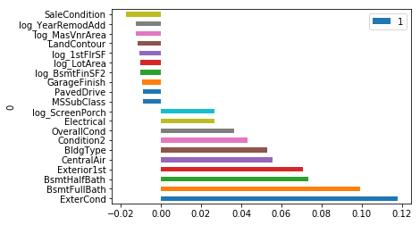
plot_coef(ridgeCV)

submission = pd.DataFrame({'SalePrice': e**ridgeCV.predict(test_scaled)},
                         index = test.index)
submission.to_csv('ames-submission-5.csv')
ridgeCV.score =  0.9540985434319784
rmsle =  0.08561971124778296


Experimentations
I tried using RobustScaler() because there are outliers in this dataset and it did not perform better.
Squaring Highly-Skewed Predictors
Although not documented here, I also tried taking a square of the log of still highly-skewed predictors, thinking deskewing those predictors more would help, and it did not.
from sklearn.preprocessing import RobustScaler
rscaler = RobustScaler()
X_rscaled = rscaler.fit_transform(X_dummies)
test_scaled = rscaler.transform(test_dummies)
lassoCV = linear_model.LassoCV()
lassoCV.fit(X_rscaled, y)
print(lassoCV.score(X_rscaled, y))

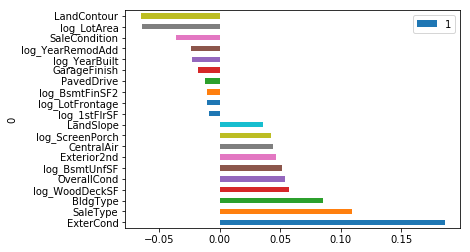
plot_coef(lassoCV)

submission = pd.DataFrame({'SalePrice': e**lassoCV.predict(test_scaled)},
                         index = test.index)
submission.to_csv('ames-submission-5.csv')
0.9362924750337854

robust scaler scoared 0.13084, not as good as 0.12890
from sklearn import linear_model
ridgeCV = linear_model.RidgeCV()
ridgeCV.fit(X_rscaled, y)
print(ridgeCV.score(X_rscaled, y))

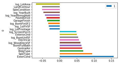
plot_coef(ridgeCV)

submission = pd.DataFrame({'SalePrice': e**ridgeCV.predict(test_scaled)},
                         index = test.index)
submission.to_csv('ames-submission-5.csv')
0.9440530646923213

robust scaler on ridge cv scored 0.12919